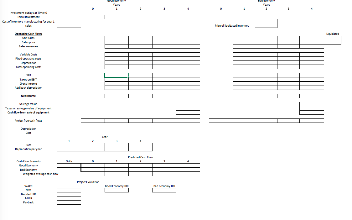
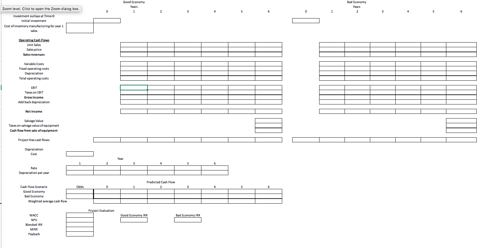
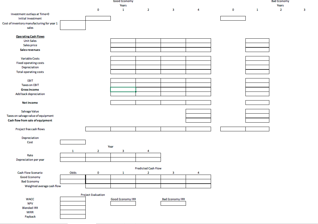
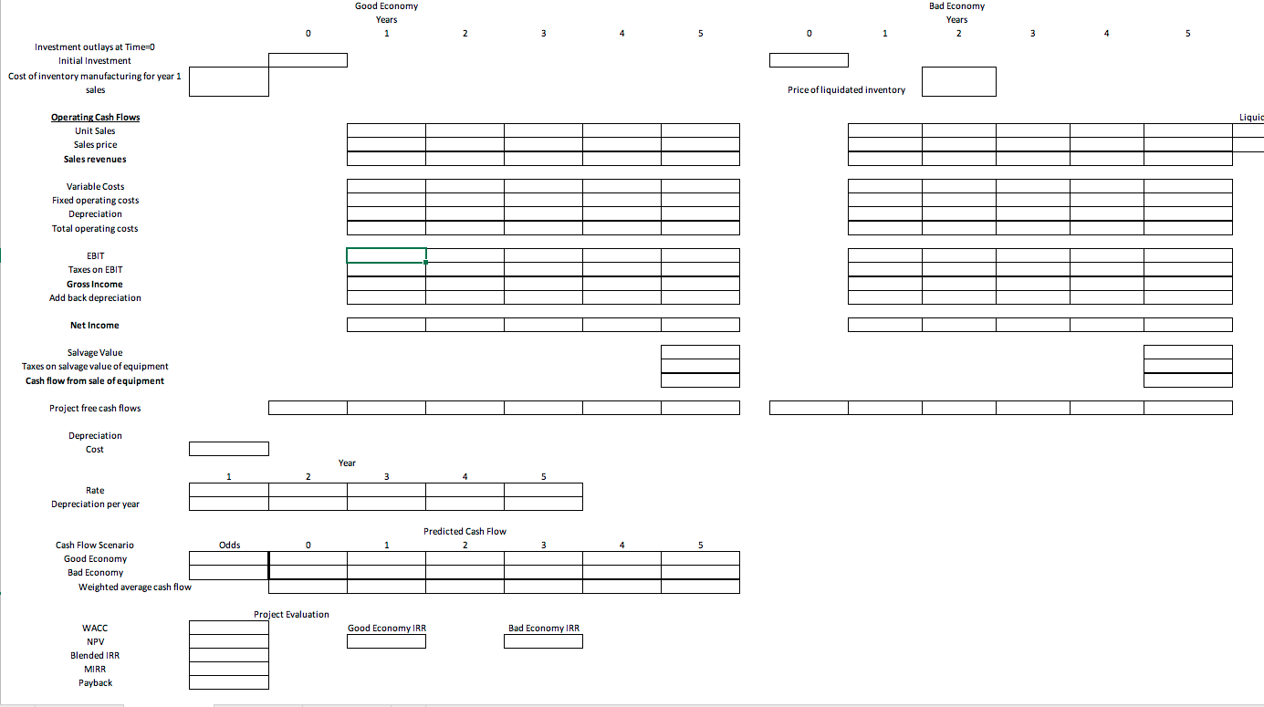Instructions Students must submit a document (MS Word file) that provides a narrative analysis of the results of their ratio calculations in their own words, not copied from annual reports. Narratives should include answers to the questions: 1. a comparison of the results of the two fiscal years for the ratios chosen (i.e., increase, decrease, ideas as to why this might have occurred) 2. a comparison to the industry average for the ratios chosen (i.e., how the company compares to the industry and what this means for the company) 3. What risk is the company facing? Is this true for the entire industry? How can the company mitigate this risk? What is the industry Beta and the company's Beta? 4. Recommendations for individuals who may be considering investing in the chosen company 5. Given the model of valuation is the company priced fairly? What recommendations would you make to increase the value of the company (be thorough make specific recommendations tied back to the company's stated financial goals). 6. Project evaluations: o Using the required rate of return calculated in part 3, evaluate the 4 projects given. To evaluate, set up the cash flow estimation in the excel spreadsheet posted, similar to table 10.4. Your company has raised $5,000,000 to invest in an expansion project(s). All 4 projects will have to begin at the same time, so evaluate the costs of the projects to check for mutually exclusiveness of the projects. Depending on the costs and returns, it is possible to invest in multiple projects. Each project will have its pros and cons, and each project to choose from will have percentages of costs and returns for Expected and Bad Economies. You will need the cash flows for each economy and do a weighted average like in Table 10.5. Set up excel using formulas. Project 2: This project is over the course of 5 years. You will need an investment of $2.5 million in Year 0, $1.75 million for equipment, and $750,000 for inventory for year 1. Depreciation is accelerated based on IRS tables (found on page 440/441 in your textbook) for special manufacturing tools, and the salvage value will be $100,000. Total inventory produced will be 15,000 units, and sales are expected to be 3,000 units per year and the final year will be the remainder of the inventory. Prices are expected to start at $700, and decrease by 15% from the prior year each year as the product ages. There is a 40% chance the Economy worsens by the end of Year 2, then sales are estimated to be 30% less then the prior year each year, prices are expected to decrease at a faster rate of 40% less than the prior year each year and inventory to be liquidated will be at a loss of 50% due to becoming obsolete. The fixed cost is $200,000 per year and the variable cost is 35% of revenue. The estimated tax rate is 40%. Project 1: This project is over the course of 4 years. You will need an investment of $5 million in year 0, $2.5 million for equipment, and $2.5 million to produce inventory for year 1. Depreciation is straight line over the 4 years, and the new equipment purchased is sold at the end of the project for a salvage value of $250,000. Fixed costs are $500,000 per year and the variable costs are 25% of sales revenues. Total inventory produced will be 85,000 units. Sales for year 1 are 15,000, year 2 are estimated to be 20,000 units at $200 each and Year 3 and 4 at 25,000 units at $125 each. The estimated tax rate is 35%. There is a 30% chance that the Economy worsens by Year 2. If so, sales are estimated to decrease 25% less than the previous year each year with no change in price after year 2 and inventory to be liquidated will be at a loss of 25%. Project 2: This project is over the course of 5 years. You will need an investment of $2.5 million in Year 0, $1.75 million for equipment, and $750,000 for inventory for year 1. Depreciation is accelerated based on IRS tables (found on page 440/441 in your textbook) for special manufacturing tools, and the salvage value will be $100,000. Total inventory produced will be 15,000 units, and sales are expected to be 3,000 units per year and the final year will be the remainder of the inventory. Prices are expected to start at $700, and decrease by 15% from the prior year each year as the product ages. There is a 40% chance the Economy worsens by the end of Year 2, then sales are estimated to be 30% less then the prior year each year, prices are expected to decrease at a faster rate of 40% less than the prior year each year and inventory to be liquidated will be at a loss of 50% due to becoming obsolete. The fixed cost is $200,000 per year and the variable cost is 35% of revenue. The estimated tax rate is 40%. Project 3: This project is over the course of 4 years. You will need an investment of $2 million in year 0, $1 million of it in inventory for year 1 production. Depreciation is a straight line over the 4 years, and the salvage value at the end of the 4 years will be $400,000. Total inventory produced will be 40,000 units, and sales are expected to be 8000 in the 1st 2 years, and 7000 in the 3rd and 4th year, with the remainder in the 4th. Prices are expected to be set at $750 for the 4 years. There is a 50% chance the new product will not receive market share by the end of the 1st year, and if that occurs, sales will only be 10% of projections in the 1st year and the price will 20% less, and the remainder of the inventory will have to be scrapped. The project will be abandoned before production starts on the second year of inventory. The machinery would be resold at the book value at the end of the 1st year. The fixed cost is $400,000 per year and the variable cost are 35% of revenue. Project 4: The tax rate is at 40%. This project is over the course of 6 years. You will need an investment of $3 million in Year 0, $1 million for equipment, and $2 million for inventory for year 1 production. Depreciation is accelerated based on IRS tables for computers from page 440/441 in your textbook, and salvage value will be $100,000. Total inventory produced will be 90,000 units, and sales are expected to be 15,000 units per year. Prices are expected to be sold to the retailers at $40. There is a 35% chance the Economy worsens after year 2, then sales are estimated to be 35% less than the previous year each year, prices will fall by 15% less than the previous year each year, and the remaining inventory at year 5 will become obsolete and destroyed. The fixed cost of creating is $200,000 per year and the variable cost is 35% of revenue. The estimated tax rate is 40%.

Good Economy Years Bad Economy Years Investment outlays at Time Initial Investment Cost of inventory manufacturing for year 1 sales Price of liquidated inventory Liquidated Operating Cash Flows Unit Sales Sales price Sales revenues Variable Costs Fixed operating costs Depreciation Total operating costs EBIT Taxes on EBIT Gross Income Add back depreciation Net Income Salvage Value Taxes on salvage value of equipment Cash flow from sale of equipment Project free cash flows Depreciation Cost Year 12 Rate Depreciation per year Predicted Cash Flow Odds 0 Cash Flow Scenario Good Economy Bad Economy Weighted average cash flow Project Evaluation Good Economy IRR Bad Economy IRR WACC NPV Blended IRR MIRR Payback Good Economy Years Bad Economy Years Zoom level. Click to open the Zoom dialog box. Investment outlays at Time=0 Initial Investment Cost of inventory manufacturing for year 1 sales Operating Cash Flows Unit Sales Sales price Sales revenues Variable Costs Fixed operating costs Depreciation Total operating costs EBIT Taxes on EBIT Gross Income Add back depreciation Net Income Salvage Value Taxes on salvage value of equipment Cash flow from sale of equipment Project free cash flows Depreciation Cost Year Rate Depreciation per year Predicted Cash Flow Odds Cash Flow Scenario Good Economy Bad Economy Weighted average cash flow Project Evaluation Good Economy IRR Bad Economy IRR WACC NPV Blended IRR MIRR Payback Bad Economy Good Economy Years Investment outlays at Time=0 Initial Investment Cost of inventory manufacturing for year 1 sales Operating Cash Flows Unit Sales Sales price Sales revenues Variable Costs Fixed operating costs Depreciation Total operating costs EBIT Taxes on EBIT Gross Income Add back depreciation Net Income Salvage Value Taxes on salvage value of equipment Cash flow from sale of equipment Project free cash flows Depreciation Cost Year 2 Rate Depreciation per year Predicted Cash Flow Odds Cash Flow Scenario Good Economy Bad Economy Weighted average cash flow Project Evaluation Good Economy IRR Bad Economy IRR WACC NPV Blended IRR MIRR Payback Good Economy Years Bad Economy Years Investment outlays at Time=0 Initial Investment Cost of inventory manufacturing for year 1 sales Price of liquidated inventory Liquic Operating Cash Flows Unit Sales Sales price Sales revenues Variable Costs Fixed operating costs Depreciation Total operating costs EBIT Taxes on EBIT Gross Income Add back depreciation Net Income Salvage Value Taxes on salvage value of equipment Cash flow from sale of equipment Project free cash flows Depreciation Cost Year Rate Depreciation per year Predicted Cash Flow Odds Cash Flow Scenario Good Economy Bad Economy Weighted average cash flow Project Evaluation Good Economy IRR Bad Economy IRR WACC NPV Blended IRR MIRR Payback Good Economy Years Bad Economy Years Investment outlays at Time Initial Investment Cost of inventory manufacturing for year 1 sales Price of liquidated inventory Liquidated Operating Cash Flows Unit Sales Sales price Sales revenues Variable Costs Fixed operating costs Depreciation Total operating costs EBIT Taxes on EBIT Gross Income Add back depreciation Net Income Salvage Value Taxes on salvage value of equipment Cash flow from sale of equipment Project free cash flows Depreciation Cost Year 12 Rate Depreciation per year Predicted Cash Flow Odds 0 Cash Flow Scenario Good Economy Bad Economy Weighted average cash flow Project Evaluation Good Economy IRR Bad Economy IRR WACC NPV Blended IRR MIRR Payback Good Economy Years Bad Economy Years Zoom level. Click to open the Zoom dialog box. Investment outlays at Time=0 Initial Investment Cost of inventory manufacturing for year 1 sales Operating Cash Flows Unit Sales Sales price Sales revenues Variable Costs Fixed operating costs Depreciation Total operating costs EBIT Taxes on EBIT Gross Income Add back depreciation Net Income Salvage Value Taxes on salvage value of equipment Cash flow from sale of equipment Project free cash flows Depreciation Cost Year Rate Depreciation per year Predicted Cash Flow Odds Cash Flow Scenario Good Economy Bad Economy Weighted average cash flow Project Evaluation Good Economy IRR Bad Economy IRR WACC NPV Blended IRR MIRR Payback Bad Economy Good Economy Years Investment outlays at Time=0 Initial Investment Cost of inventory manufacturing for year 1 sales Operating Cash Flows Unit Sales Sales price Sales revenues Variable Costs Fixed operating costs Depreciation Total operating costs EBIT Taxes on EBIT Gross Income Add back depreciation Net Income Salvage Value Taxes on salvage value of equipment Cash flow from sale of equipment Project free cash flows Depreciation Cost Year 2 Rate Depreciation per year Predicted Cash Flow Odds Cash Flow Scenario Good Economy Bad Economy Weighted average cash flow Project Evaluation Good Economy IRR Bad Economy IRR WACC NPV Blended IRR MIRR Payback Good Economy Years Bad Economy Years Investment outlays at Time=0 Initial Investment Cost of inventory manufacturing for year 1 sales Price of liquidated inventory Liquic Operating Cash Flows Unit Sales Sales price Sales revenues Variable Costs Fixed operating costs Depreciation Total operating costs EBIT Taxes on EBIT Gross Income Add back depreciation Net Income Salvage Value Taxes on salvage value of equipment Cash flow from sale of equipment Project free cash flows Depreciation Cost Year Rate Depreciation per year Predicted Cash Flow Odds Cash Flow Scenario Good Economy Bad Economy Weighted average cash flow Project Evaluation Good Economy IRR Bad Economy IRR WACC NPV Blended IRR MIRR Payback