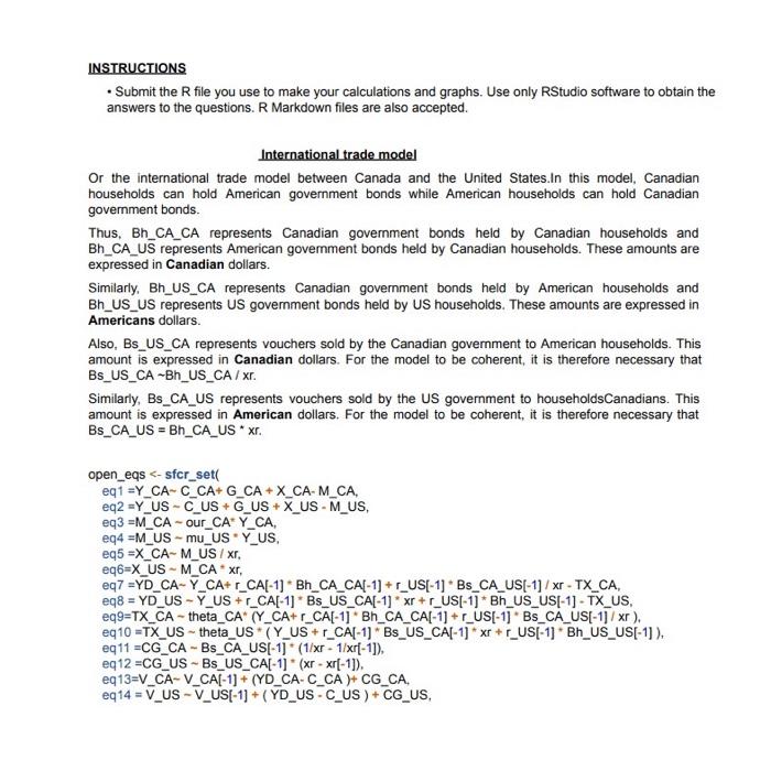
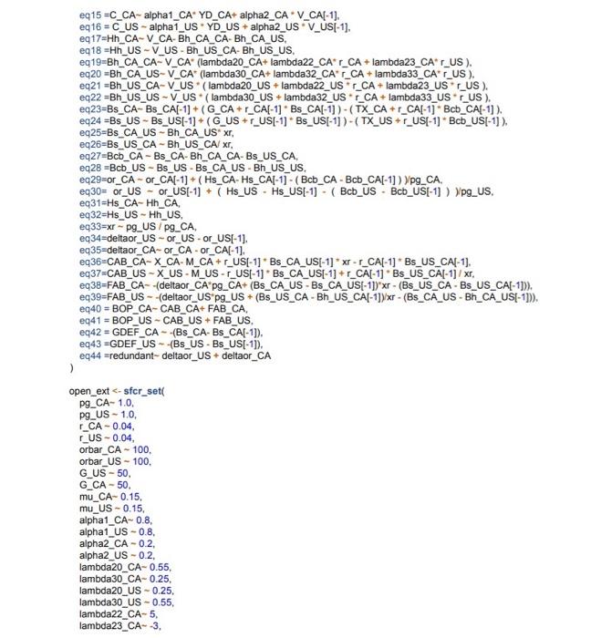
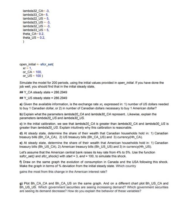
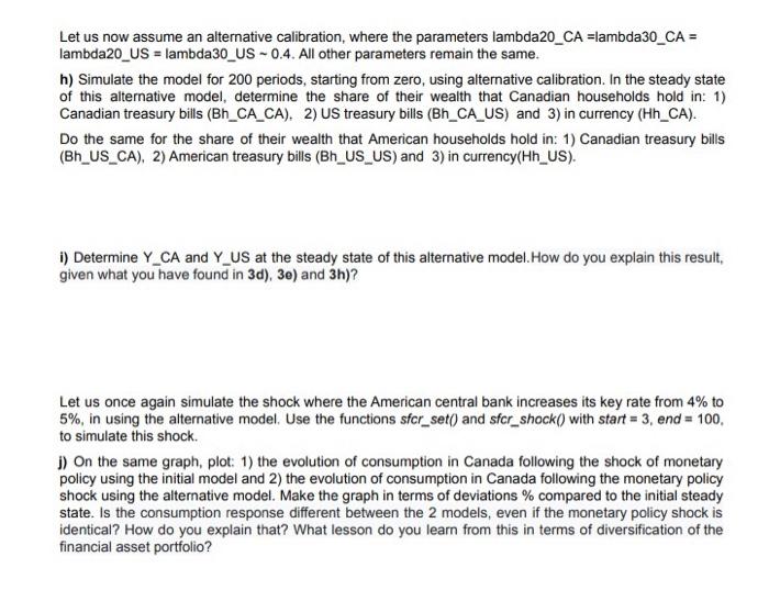
INSTRUCTIONS - Submit the R file you use to make your calculations and graphs. Use only RStudio software to obtain the answers to the questions. R Markdown files are also accepted. International trade model Or the international trade model between Canada and the United States.In this model, Canadian households can hold American government bonds while American households can hold Canadian government bonds. Thus, Bh_CA_CA represents Canadian government bonds held by Canadian households and Bh_CA_US represents American govemment bonds held by Canadian households. These amounts are expressed in Canadian dollars. Similarly, Bh_US_CA represents Canadian government bonds held by American households and Bh_US_US represents US government bonds held by US households. These amounts are expressed in Americans dollars. Also, Bs_US_CA represents vouchers sold by the Canadian government to American households. This amount is expressed in Canadian dollars. For the model to be coherent, it is therefore necessary that Bs_US_CA Bh_US_CA / xr. Similarly, Bs_CA_US represents vouchers sold by the US government to householdsCanadians. This amount is expressed in American dollars. For the model to be coherent, it is therefore necessary that Bs_CA_US = Bh_CA_US * x. open_eqs 1=Y_CAC_CA+G_CA+X_CAM_CA, eq 2=Y Y_US C_US+G_US+X_USM_US, eq 3= M_CA - our_CA YC, eq4 4 M_US - mu_US * Y_US, eq5 = X_CA M_US /xr. eq 6=X _US MCCAx, eq 7 =YD_CA Y_CA+r_CA[1] * Bh_CA_CA[-1] + r_US[-1] * Bs_CA_US[-1] / xr - TX_CA, eq 11= CG_CA - Bs_CA_US[-1] (1/xr1/xr[1]), eq 12 =CG_US Bs_US_CA[-1] * (xr - xr[-1]). eq 13=VCAVCA[1]+(YD_CAC_CA)+C_CA, eq14 =V _US V_US[1]+( YD_US CUS)+C _ US , eq15 =C_CA - alpha1_CA*YD_CA+ alpha2_CA * V_CA [1], eq1 16 = C_US - alpha1_US * YD_US + alph2_US * V_US[-1], eq 17=Hh _CA V_CAB _ CA_CA-Bh_CA_US, eq 18= Hh_US V _US - Bh_US_CA-Bh_US_US. eq19 Bh_CA_CA - V_CA* (lambda20_CA+lambda22_CA* r_CA + lambda23_CA* r_uS ). eq21 =Bh_US_CA - V_US * ( lambda20_US + lambda22_US *r_CA + lambda23_US*r_US ). eq22 =Bh_US_US - V_US * ( lambda30_US + lambda32_US * r_CA + lambda33_US * r_US ). eq 25= Bs_CA_US - Bh_CA_US* x, eq 26= Bs_US_CA - Bh_US_CA /xr, eq 27= Bcb_CA - Bs_CA - Bh_CA_CA-Bs_US_CA, eq2 28=Bcb_US - Bs_US - Bs_CA_US - Bh_US_US. eq29 = or_CA - or_CA [1]+(HsCAHsCA[1](BcbCABcbCA[1])) pg_CA. eq31=Hs_CA- Hh_CA. eq 32=Hs _US Hh2 US, eq 33=xr pg_US / pg_CA, eq 34= deltaor_US - or_US - or_US[-1]. eq 35= deltaor_CA - or_CA - or_CA[-1], eq 36= CAB_CA - X_CA - M_CA + r_US[-1] *Bs_CA_US[-1] * xr - r_CA[-1] * Bs_US_CA[-1], eq39=FAB_US - -(deltaor_US'pg_US + (Bs_US_CA - Bh_US_CA[-1])/xr - (Bs_CA_US - Bh_CA_US[-1])). eq40 = BOP CA - CAB_CA + FAB_CA, eq4 41= BOP_US - CAB_US + FAB B US. eq43 =GDEF_US - (Bs_US - Bs_US[-1]). eq44 =redundant - deltaor_US + deltaor_CA ) open_ext CA0.04, rUS - 0.04, orbar_CA -100 . orbar_US - 100 . G_US -50 , G_CA - 50 . mu_CA-0.15. mu_US - 0.15 , alpha1_CA 0.8, alpha1_US - 0.8, alpha2_CA -0.2 , alpha2_US - 0.2, lambda20_CA-0.55, lambda30_CA 0.25 , lambda20_US 0.25, lambda30_US - 0.55, lambda22_CA-5, lambda23_CA- 3 , \[ \begin{array}{l} \text { lambda32_CA }-3 \text {, } \\ \text { lambda33_CA }-5 \text {, } \\ \text { lambda22_US }-5 \text {, } \\ \text { lambda23_US }-3 \text {, } \\ \text { lambda32_US } \sim-3 \text {, } \\ \text { lambda33_US } \sim 5 \text {, } \\ \text { theta_CA } 0.2, \\ \text { theta_US }-0.2, \\ \text { l } \end{array} \] \[ \begin{array}{l} \text { open_initial =286.2949 \#_ Y_US steady state =286.2949 a) Given the available information, is the exchange rate xt expressed in: 1) number of US dollars needed to buy 1 Canadian dollar, or 2) in number of Canadian dollars necessary to buy 1 American dollar? b) Explain what the parameters lambda20_CA and lambda30_CA represent. Likewise, explain the parameters lambda20_US and lambda30_US. c) In the initial calibration, we see that lambda20_CA is greater than lambda30_CA and lambda30_US is greater than lambda20_US. Explain intuitively why this calibration is reasonable. d) At steady state, determine the share of their wealth that Canadian households hold in: 1) Canadian treasury bills (Bh_CA_CA), 2) US treasury bills (Bh_CA_US) and 3) currency(Hh_CA). e) At steady state, determine the share of their wealth that American households hold in: 1) Canadian treasury bills (Bh_US_CA). 2) American treasury bills (Bh_US_US) and 3) in currency(Hh_US). Let's assume that the American central bank raises its key rate from 4% to 5%. Use the function ssfcr_set() and sfcr_shock() with start =3, end =100, to simulate this shock. f) Draw on the same graph the evolution of consumption in Canada and the USA following this shock. Make the graph in terms of % deviation from the initial steady state. Which country gains the most from this change in the American interest rate? g) Plot Bh_CA_CA and Bh_CA_US on the same graph. And on a different chart plot Bh_US_CA and Bh_US_US. Which government securities are seeing increasing demand? Which government securities are seeing its demand decrease? How do you explain the behavior of these variables? Let us now assume an alternative calibration, where the parameters lambda20_CA =lambda30_CA = lambda20_US = lambda30_US 0.4. All other parameters remain the same. h) Simulate the model for 200 periods, starting from zero, using alternative calibration. In the steady state of this alternative model, determine the share of their wealth that Canadian households hold in: 1) Canadian treasury bills (Bh_CA_CA), 2) US treasury bills (Bh_CA_US) and 3) in currency (Hh_CA). Do the same for the share of their wealth that American households hold in: 1) Canadian treasury bills (Bh_US_CA), 2) American treasury bills (Bh_US_US) and 3) in currency(Hh_US). i) Determine YCA and YUS at the steady state of this alternative model. How do you explain this result, given what you have found in 3d),3e ) and 3h )? Let us once again simulate the shock where the American central bank increases its key rate from 4% to 5%, in using the alternative model. Use the functions sfcr_set() and sfcr_shock() with start =3, end =100, to simulate this shock. j) On the same graph, plot: 1) the evolution of consumption in Canada following the shock of monetary policy using the initial model and 2) the evolution of consumption in Canada following the monetary policy shock using the alternative model. Make the graph in terms of deviations \% compared to the initial steady state. Is the consumption response different between the 2 models, even if the monetary policy shock is identical? How do you explain that? What lesson do you learn from this in terms of diversification of the financial asset portfolio


