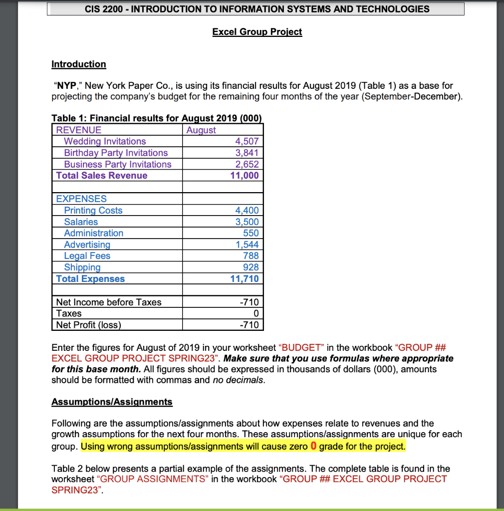
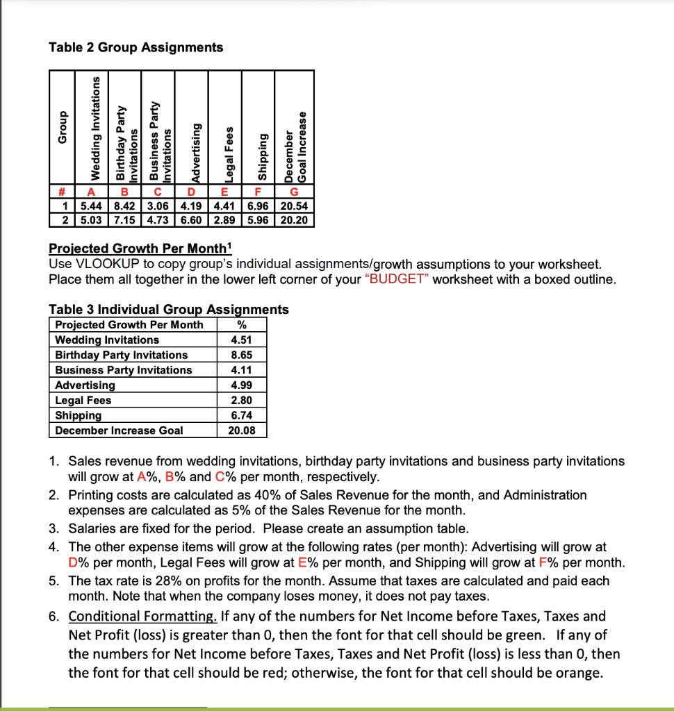
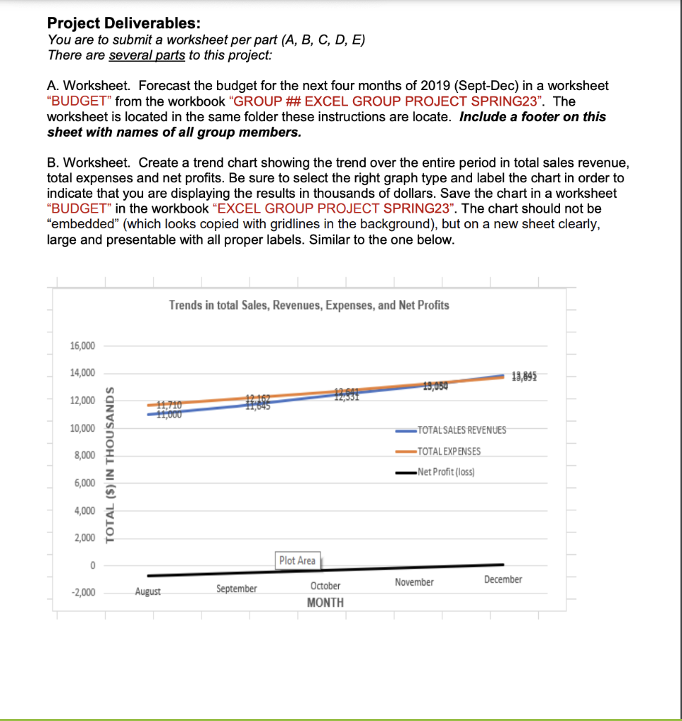
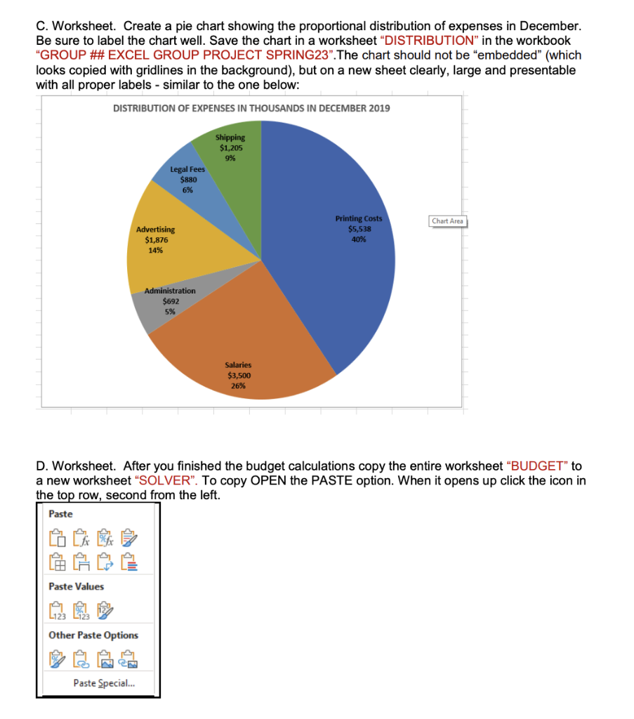
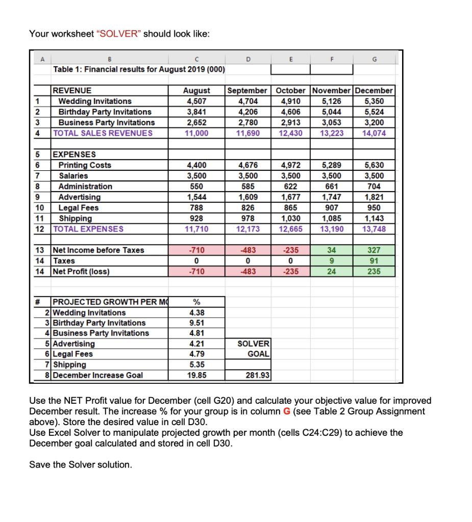
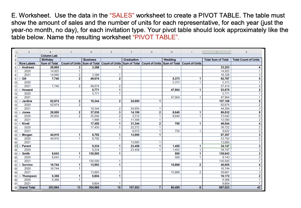
Introduction "NYP," New York Paper Co., is using its financial results for August 2019 (Table 1) as a base for projecting the company's budget for the remaining four months of the year (September-December). Enter the figures for August of 2019 in your worksheet "BUDGET" in the workbook "GROUP \#\# EXCEL GROUP PROJECT SPRING23". Make sure that you use formulas where appropriate for this base month. All figures should be expressed in thousands of dollars (000), amounts should be formatted with commas and no decimals. Assumptions/Assignments Following are the assumptions/assignments about how expenses relate to revenues and the growth assumptions for the next four months. These assumptions/assignments are unique for each group. Using wrong assumptions/assignments will cause zero 0 grade for the project. Table 2 below presents a partial example of the assignments. The complete table is found in the worksheet "GROUP ASSIGNMENTS" in the workbook "GROUP \#\# EXCEL GROUP PROJECT SPRING23". Table 2 Group Assignments Projected Growth Per Month 1 Use VLOOKUP to copy group's individual assignments/growth assumptions to your worksheet. Place them all together in the lower left corner of your "BUDGET" worksheet with a boxed outline. Tahle 3 Individual Groun Assionments 1. Sales revenue from wedding invitations, birthday party invitations and business party invitations will grow at A%,B% and C% per month, respectively. 2. Printing costs are calculated as 40% of Sales Revenue for the month, and Administration expenses are calculated as 5% of the Sales Revenue for the month. 3. Salaries are fixed for the period. Please create an assumption table. 4. The other expense items will grow at the following rates (per month): Advertising will grow at D% per month, Legal Fees will grow at E% per month, and Shipping will grow at F% per month. 5. The tax rate is 28% on profits for the month. Assume that taxes are calculated and paid each month. Note that when the company loses money, it does not pay taxes. 6. Conditional Formatting. If any of the numbers for Net Income before Taxes, Taxes and Net Profit (loss) is greater than 0 , then the font for that cell should be green. If any of the numbers for Net Income before Taxes, Taxes and Net Profit (loss) is less than 0, then the font for that cell should be red; otherwise, the font for that cell should be orange. Project Deliverables: You are to submit a worksheet per part (A,B,C,D,E) There are several parts to this project: A. Worksheet. Forecast the budget for the next four months of 2019 (Sept-Dec) in a worksheet "BUDGET" from the workbook "GROUP \#\# EXCEL GROUP PROJECT SPRING23". The worksheet is located in the same folder these instructions are locate. Include a footer on this sheet with names of all group members. B. Worksheet. Create a trend chart showing the trend over the entire period in total sales revenue, total expenses and net profits. Be sure to select the right graph type and label the chart in order to indicate that you are displaying the results in thousands of dollars. Save the chart in a worksheet "BUDGET" in the workbook "EXCEL GROUP PROJECT SPRING23". The chart should not be "embedded" (which looks copied with gridlines in the background), but on a new sheet clearly, large and presentable with all proper labels. Similar to the one below. C. Worksheet. Create a pie chart showing the proportional distribution of expenses in December. Be sure to label the chart well. Save the chart in a worksheet "DISTRIBUTION" in the workbook "GROUP \#\# EXCEL GROUP PROJECT SPRING23". The chart should not be "embedded" (which looks copied with gridlines in the background), but on a new sheet clearly, large and presentable with all proper labels - similar to the one below: D. Worksheet. After you finished the budget calculations copy the entire worksheet "BUDGET" to a new worksheet "SOLVER". To copy OPEN the PASTE option. When it opens up click the icon in the top row, second from the left. Your worksheet "SOLVER" should look like: Use the NET Profit value for December (cell G20) and calculate your objective value for improved December result. The increase \% for your group is in column G (see Table 2 Group Assignment above). Store the desired value in cell D30. Use Excel Solver to manipulate projected growth per month (cells C24:C29) to achieve the December goal calculated and stored in cell D30. Save the Solver solution. E. Worksheet. Use the data in the "SALES" worksheet to create a PIVOT TABLE. The table must show the amount of sales and the number of units for each representative, for each year (just the year-no month, no day), for each invitation type. Your pivot table should look approximately like the table below. Name the resulting worksheet "PIVOT TABLE". Very Important Final Notes: Include a footer on every worksheet with names of all group members. Delete any extra sheets that are not to be graded especially if they are blank > All worksheets should be submitted as 1 (one) workbook via Blackboard before the due date. The name of the workbook file should be (GROUP \#\# EXCEL GROUP PROJECT SPRING23). Include your group \#\# (e.g., 23, 04, 15, etc.) to get the credit. Files that do not follow this naming convention will receive a reduced grade (10%). > Your workbook should look professional to earn the highest grade. You should do a print preview to make sure that everything is formatted properly and looks presentable. > Assume this will be opened on a Windows computer. Therefore, it should be tested prior to submitting. You have 2 attempts to submit your project - I will grade the latest attempt only. You will lose points if you submit an incomplete or erroneous project. Don't wait for the last few days to complete this assignment. Please don't email me your assignment for "checking". GRADING RUBRICS You start with 100% for each worksheet. The grade will be reduced as follows: BUDGET - incorrect/missing formulas; hard coded numbers; incorrect formatting and conditional formatting; incorrectly copied assignments/assumptions. TREND CHART - incorrect chart; missing/incorrect labels, titles, legend. PIE CHART - incorrect chart; missing/incorrect labels, titles, legend. SOLVER - incorrect formula, incorrect objective, incorrect variables PIVOT TABLE - hard coded table, incomplete table, incorrect fields, required information is missing. Introduction "NYP," New York Paper Co., is using its financial results for August 2019 (Table 1) as a base for projecting the company's budget for the remaining four months of the year (September-December). Enter the figures for August of 2019 in your worksheet "BUDGET" in the workbook "GROUP \#\# EXCEL GROUP PROJECT SPRING23". Make sure that you use formulas where appropriate for this base month. All figures should be expressed in thousands of dollars (000), amounts should be formatted with commas and no decimals. Assumptions/Assignments Following are the assumptions/assignments about how expenses relate to revenues and the growth assumptions for the next four months. These assumptions/assignments are unique for each group. Using wrong assumptions/assignments will cause zero 0 grade for the project. Table 2 below presents a partial example of the assignments. The complete table is found in the worksheet "GROUP ASSIGNMENTS" in the workbook "GROUP \#\# EXCEL GROUP PROJECT SPRING23". Table 2 Group Assignments Projected Growth Per Month 1 Use VLOOKUP to copy group's individual assignments/growth assumptions to your worksheet. Place them all together in the lower left corner of your "BUDGET" worksheet with a boxed outline. Tahle 3 Individual Groun Assionments 1. Sales revenue from wedding invitations, birthday party invitations and business party invitations will grow at A%,B% and C% per month, respectively. 2. Printing costs are calculated as 40% of Sales Revenue for the month, and Administration expenses are calculated as 5% of the Sales Revenue for the month. 3. Salaries are fixed for the period. Please create an assumption table. 4. The other expense items will grow at the following rates (per month): Advertising will grow at D% per month, Legal Fees will grow at E% per month, and Shipping will grow at F% per month. 5. The tax rate is 28% on profits for the month. Assume that taxes are calculated and paid each month. Note that when the company loses money, it does not pay taxes. 6. Conditional Formatting. If any of the numbers for Net Income before Taxes, Taxes and Net Profit (loss) is greater than 0 , then the font for that cell should be green. If any of the numbers for Net Income before Taxes, Taxes and Net Profit (loss) is less than 0, then the font for that cell should be red; otherwise, the font for that cell should be orange. Project Deliverables: You are to submit a worksheet per part (A,B,C,D,E) There are several parts to this project: A. Worksheet. Forecast the budget for the next four months of 2019 (Sept-Dec) in a worksheet "BUDGET" from the workbook "GROUP \#\# EXCEL GROUP PROJECT SPRING23". The worksheet is located in the same folder these instructions are locate. Include a footer on this sheet with names of all group members. B. Worksheet. Create a trend chart showing the trend over the entire period in total sales revenue, total expenses and net profits. Be sure to select the right graph type and label the chart in order to indicate that you are displaying the results in thousands of dollars. Save the chart in a worksheet "BUDGET" in the workbook "EXCEL GROUP PROJECT SPRING23". The chart should not be "embedded" (which looks copied with gridlines in the background), but on a new sheet clearly, large and presentable with all proper labels. Similar to the one below. C. Worksheet. Create a pie chart showing the proportional distribution of expenses in December. Be sure to label the chart well. Save the chart in a worksheet "DISTRIBUTION" in the workbook "GROUP \#\# EXCEL GROUP PROJECT SPRING23". The chart should not be "embedded" (which looks copied with gridlines in the background), but on a new sheet clearly, large and presentable with all proper labels - similar to the one below: D. Worksheet. After you finished the budget calculations copy the entire worksheet "BUDGET" to a new worksheet "SOLVER". To copy OPEN the PASTE option. When it opens up click the icon in the top row, second from the left. Your worksheet "SOLVER" should look like: Use the NET Profit value for December (cell G20) and calculate your objective value for improved December result. The increase \% for your group is in column G (see Table 2 Group Assignment above). Store the desired value in cell D30. Use Excel Solver to manipulate projected growth per month (cells C24:C29) to achieve the December goal calculated and stored in cell D30. Save the Solver solution. E. Worksheet. Use the data in the "SALES" worksheet to create a PIVOT TABLE. The table must show the amount of sales and the number of units for each representative, for each year (just the year-no month, no day), for each invitation type. Your pivot table should look approximately like the table below. Name the resulting worksheet "PIVOT TABLE". Very Important Final Notes: Include a footer on every worksheet with names of all group members. Delete any extra sheets that are not to be graded especially if they are blank > All worksheets should be submitted as 1 (one) workbook via Blackboard before the due date. The name of the workbook file should be (GROUP \#\# EXCEL GROUP PROJECT SPRING23). Include your group \#\# (e.g., 23, 04, 15, etc.) to get the credit. Files that do not follow this naming convention will receive a reduced grade (10%). > Your workbook should look professional to earn the highest grade. You should do a print preview to make sure that everything is formatted properly and looks presentable. > Assume this will be opened on a Windows computer. Therefore, it should be tested prior to submitting. You have 2 attempts to submit your project - I will grade the latest attempt only. You will lose points if you submit an incomplete or erroneous project. Don't wait for the last few days to complete this assignment. Please don't email me your assignment for "checking". GRADING RUBRICS You start with 100% for each worksheet. The grade will be reduced as follows: BUDGET - incorrect/missing formulas; hard coded numbers; incorrect formatting and conditional formatting; incorrectly copied assignments/assumptions. TREND CHART - incorrect chart; missing/incorrect labels, titles, legend. PIE CHART - incorrect chart; missing/incorrect labels, titles, legend. SOLVER - incorrect formula, incorrect objective, incorrect variables PIVOT TABLE - hard coded table, incomplete table, incorrect fields, required information is missing