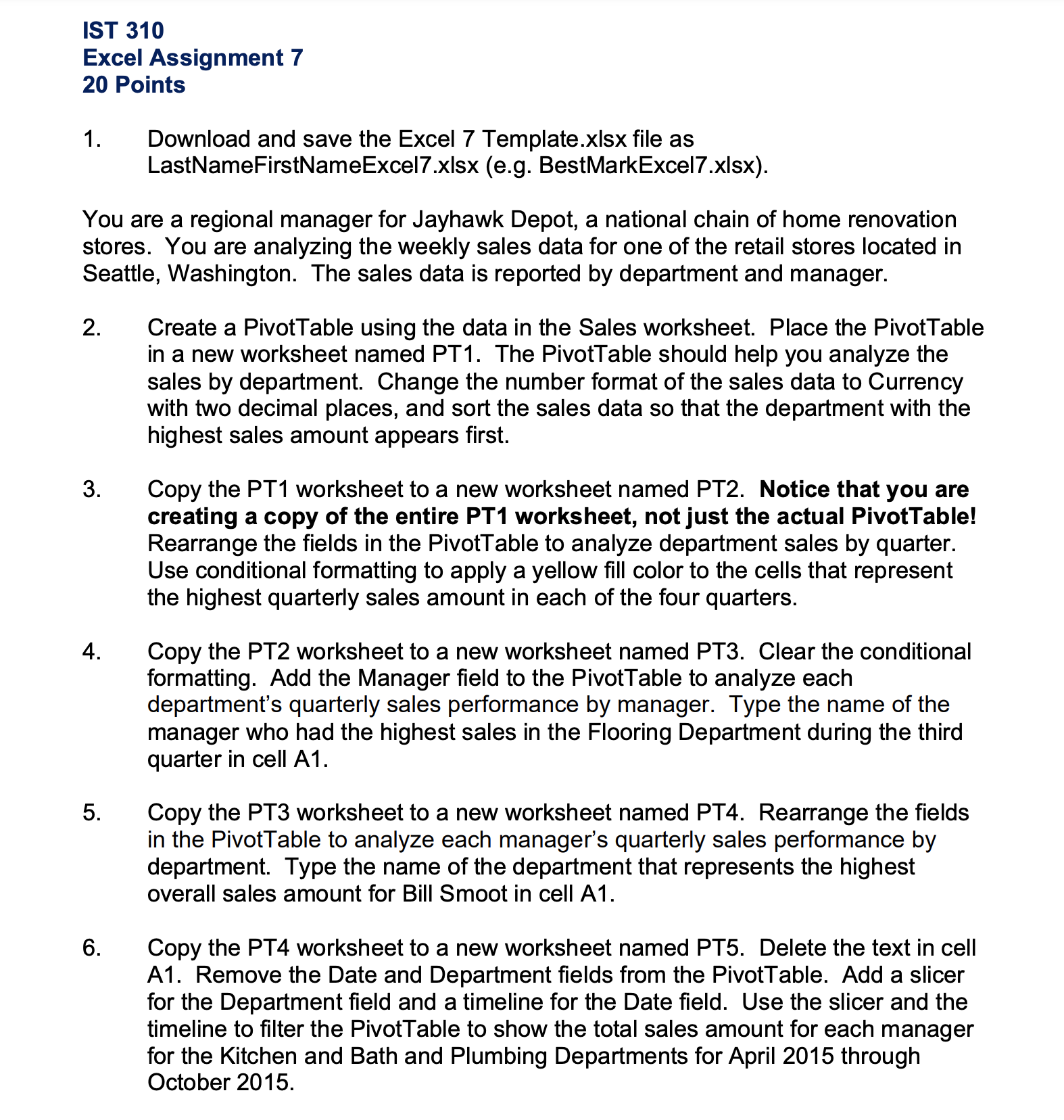
IST 310 Excel Assignment 7 20 Points 1. Download and save the Excel 7 Template.xlsx file as LastNameFirstNameExcel7.xlsx (e.g. BestMarkExcel7.xlsx). You are a regional manager for Jayhawk Depot, a national chain of home renovation stores. You are analyzing the weekly sales data for one of the retail stores located in Seattle, Washington. The sales data is reported by department and manager. 2. 3. 4. 5. 6. Create a PivotTable using the data in the Sales worksheet. Place the PivotTable in a new worksheet named PT1. The PivotTable should help you analyze the sales by department. Change the number format of the sales data to Currency with two decimal places, and sort the sales data so that the department with the highest sales amount appears first. Copy the PT1 worksheet to a new worksheet named PT2. Notice that you are creating a copy of the entire PT1 worksheet, not just the actual PivotTable! Rearrange the fields in the PivotTable to analyze department sales by quarter. Use conditional formatting to apply a yellow fill color to the cells that represent the highest quarterly sales amount in each of the four quarters. Copy the PT2 worksheet to a new worksheet named PT3. Clear the conditional formatting. Add the Manager field to the PivotTable to analyze each department's quarterly sales performance by manager. Type the name of the manager who had the highest sales in the Flooring Department during the third quarter in cell A1. Copy the PT3 worksheet to a new worksheet named PT4. Rearrange the fields in the PivotTable to analyze each manager's quarterly sales performance by department. Type the name of the department that represents the highest overall sales amount for Bill Smoot in cell A1. Copy the PT4 worksheet to a new worksheet named PT5. Delete the text in cell A1. Remove the Date and Department fields from the PivotTable. Add a slicer for the Department field and a timeline for the Date field. Use the slicer and the timeline to filter the PivotTable to show the total sales amount for each manager for the Kitchen and Bath and Plumbing Departments for April 2015 through October 2015.