I've answer problem #1 with this

n = 0:1:999; %vector 0 to 999 a = .6; %alpha value z = 1; %z value xn = a.^n; %function within the given range xz1 = sum(xn.*z.^(-n)); %fianl z-transform equation

But now I have to use the answer in problem #1 to answer problem #3.

I need a guideline on how to code #3

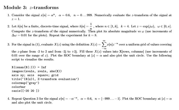
Module 3: z-transforms 1. Consider the signal [n] = 0", a=0.6, n=0...999. Numerically evaluate the z-transform of the signal at z=1. 2. Let h[n] be a finite, discrete-time signal, where h[n] = =, where ne [1,k), k= 4. Let 2 = exp(jw), we [0,w). Compute the z-transform of the signal numerically. Then plot its absolute magnitude vs w (use increments of Aw = 0.01 for the plots). Repeat the experiment for k=8. 3. For the signal in (1), evaluate X (2) using the definition X(z) = x[n]2 -" over a uniform grid of values covering the 2-plane from -2 to 2 and from -2j to +2j. Fill these X(2) values into X[rows, columns (use increments of 0.01 over the range of ). Plot the ROC boundary at 1:1 = x and also plot the unit circle. Use the following script to visualize the results. X(isnan (X(:))) - Inf imagesc (zvals, zvals, abs(x)) axis xy: axis square; grid title('|x(z)I, Z-transform evaluation') colormap('gray') colorbar caxis((-20 20 ]) 4. Repeat Question 3 for the signal [n] = -a-", a=0.6, n= [-999...-1). Plot the ROC boundary at 1:1 = a and also plot the unit circle. Module 3: z-transforms 1. Consider the signal [n] = 0", a=0.6, n=0...999. Numerically evaluate the z-transform of the signal at z=1. 2. Let h[n] be a finite, discrete-time signal, where h[n] = =, where ne [1,k), k= 4. Let 2 = exp(jw), we [0,w). Compute the z-transform of the signal numerically. Then plot its absolute magnitude vs w (use increments of Aw = 0.01 for the plots). Repeat the experiment for k=8. 3. For the signal in (1), evaluate X (2) using the definition X(z) = x[n]2 -" over a uniform grid of values covering the 2-plane from -2 to 2 and from -2j to +2j. Fill these X(2) values into X[rows, columns (use increments of 0.01 over the range of ). Plot the ROC boundary at 1:1 = x and also plot the unit circle. Use the following script to visualize the results. X(isnan (X(:))) - Inf imagesc (zvals, zvals, abs(x)) axis xy: axis square; grid title('|x(z)I, Z-transform evaluation') colormap('gray') colorbar caxis((-20 20 ]) 4. Repeat Question 3 for the signal [n] = -a-", a=0.6, n= [-999...-1). Plot the ROC boundary at 1:1 = a and also plot the unit circle