Japan experienced impressive rates of growth, especially between 1950 and 1975. As depicted in the figure below, this experience was enough to bring the levels of GDP per worker closer to the US in about four decades

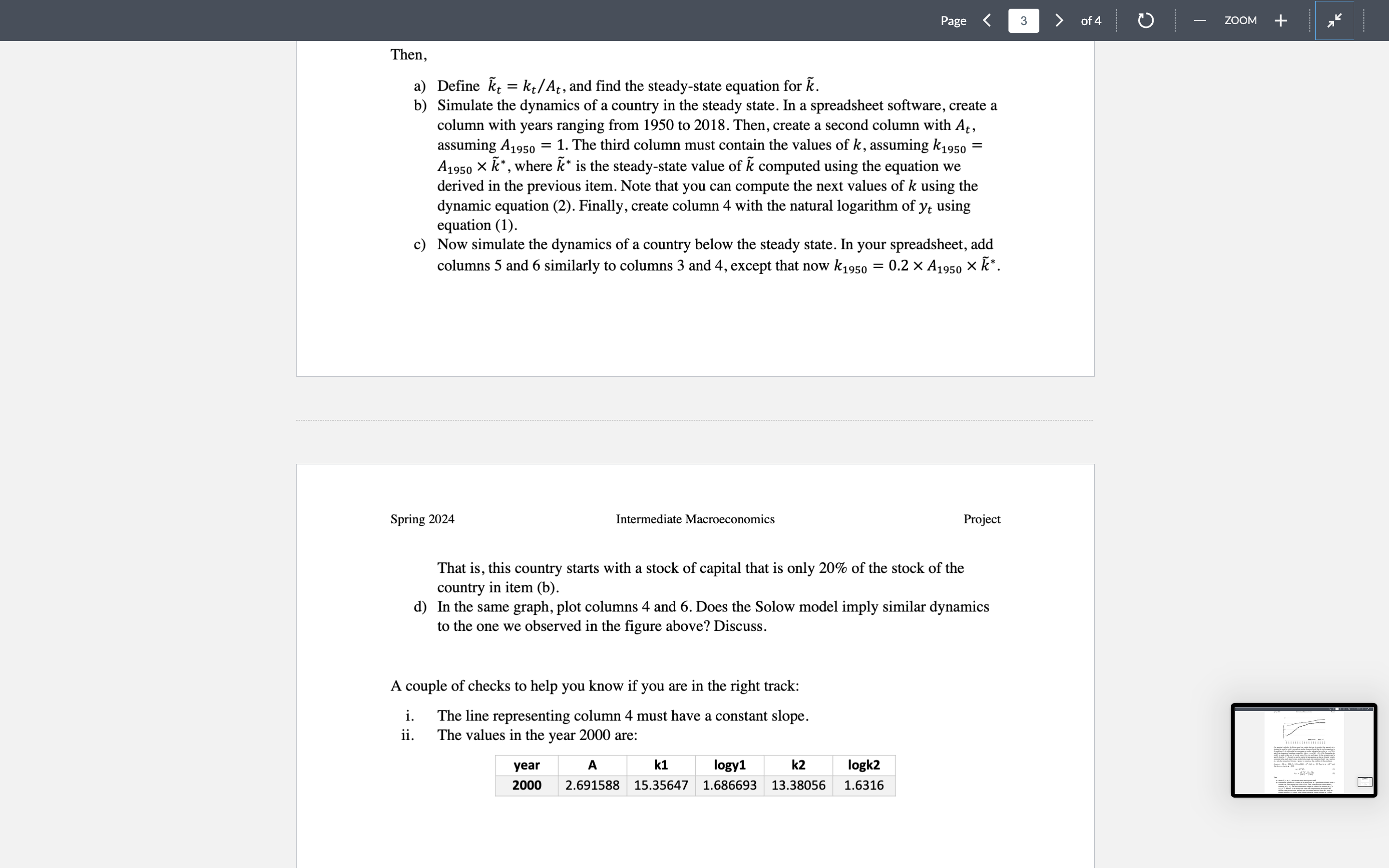
One question is whether the Solow model can explain this type of miracles. One approach is to simulate the model to test if it can replicate similar dynamics. Recall that the two key equations in the model are (1) the relationship between output per worker and capital per worker ?? = ???(??), and (2) the dynamics of capital per worker (1 + ?)??+1 = ????(??) + (1 ? ?)??. To simulate the model, we need to take care of several issues. First, we need values for the parameters and a specific form for ?(?). Second, we need to rewrite the key equations so that our dynamic variable is constant in the steady state. In class, we derived a steady-state condition where ? was a function of ? and other parameters. But since ? grows, we cannot use that condition for the simulation. Assume ? = 0.2, ? = 0.02, ? = 0.03, and ?(?) = ?? which ? = 0.4. Then, let ?? = ?? 1?? such that ?? grows at a rate ? = 0.02.

?? = ?? 1???? ?, (1) ??+1 = ??? 1???? ? (1 + ?) + (1 ? ?)?? (1 + ?) . (2) Then, a) Define ??? = ?? ??? , and find the steady-state equation for ?? . b) Simulate the dynamics of a country in the steady state. In a spreadsheet software, create a column with years ranging from 1950 to 2018. Then, create a second column with ??, assuming ?1950 = 1. The third column must contain the values of ?, assuming ?1950 = ?1950 ?? ?, where ?? ? is the steady-state value of ?? computed using the equation we derived in the previous item. Note that you can compute the next values of ? using the dynamic equation (2). Finally, create column 4 with the natural logarithm of ?? using equation (1). c) Now simulate the dynamics of a country below the steady state. In your spreadsheet, add columns 5 and 6 similarly to columns 3 and 4, except that now ?1950 = 0.2 ?1950 ?? ?. 8 9 10 11 12 1950 1954 1958 1962 1966 1970 1974 1978 1982 1986 1990 1994 1998 2002 2006 2010 2014 2018 log(Per Worker GDP) Japan US

d) In the same graph, plot columns 4 and 6. Does the Solow model imply similar dynamics to the one we observed in the figure above? Discuss

=R B O zooM + Then, a) Define k; = k;/A,,and find the steady-state equation for k. b) Simulate the dynamics of a country in the steady state. In a spreadsheet software, create a column with years ranging from 1950 to 2018. Then, create a second column with 4,, assuming A;g50 = 1. The third column must contain the values of k, assuming k959 = Aqoso X k*, where k* is the steady-state value of k computed using the equation we derived in the previous item. Note that you can compute the next values of k using the dynamic equation (2). Finally, create column 4 with the natural logarithm of y, using equation (1). c) Now simulate the dynamics of a country below the steady state. In your spreadsheet, add columns 5 and 6 similarly to columns 3 and 4, except that now kjg59 = 0.2 X Aj950 X k. Spring 2024 Intermediate Macroeconomics Project That is, this country starts with a stock of capital that is only 20% of the stock of the country in item (b). d) In the same graph, plot columns 4 and 6. Does the Solow model imply similar dynamics to the one we observed in the figure above? Discuss. A couple of checks to help you know if you are in the right track: i. The line representing column 4 must have a constant slope. ii. The values in the year 2000 are: year A k1 logyl k2 logk2 2000 2.691588 15.35647 1.686693 13.38056 1.6316