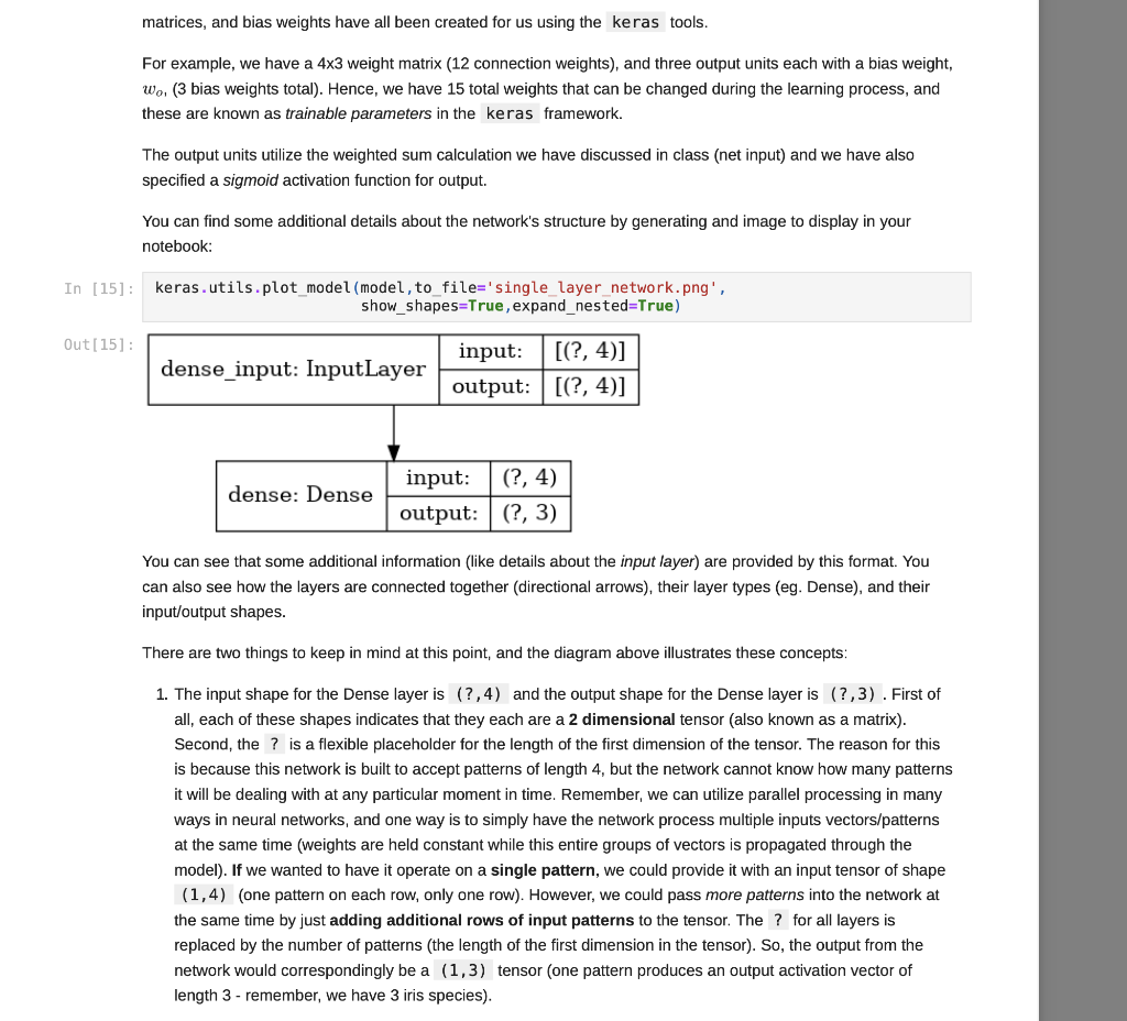
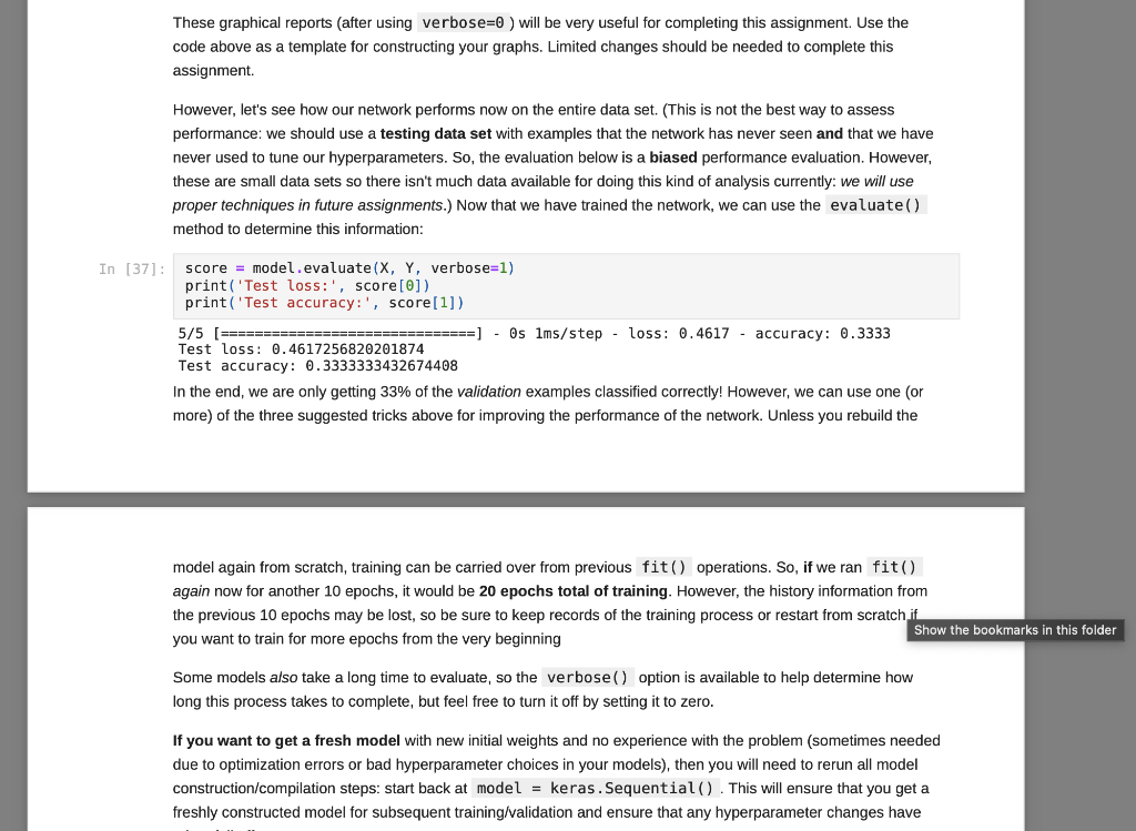
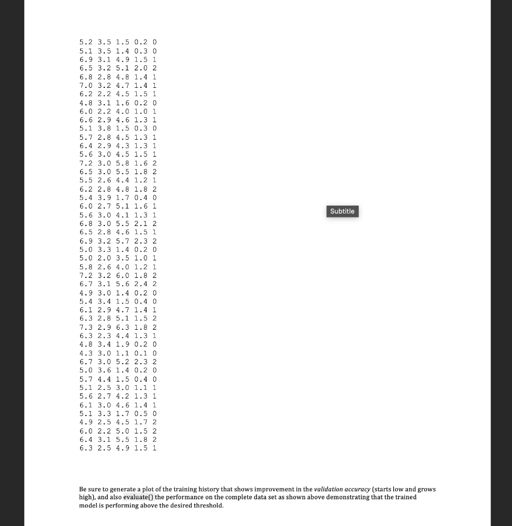
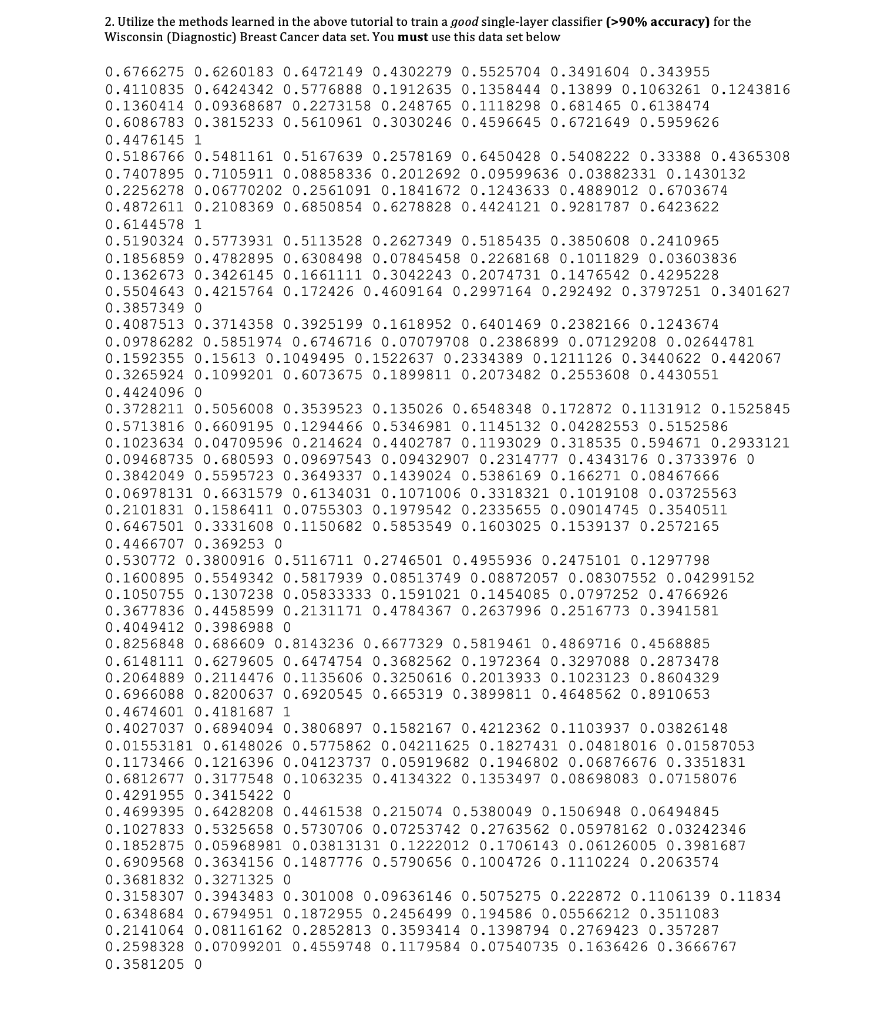
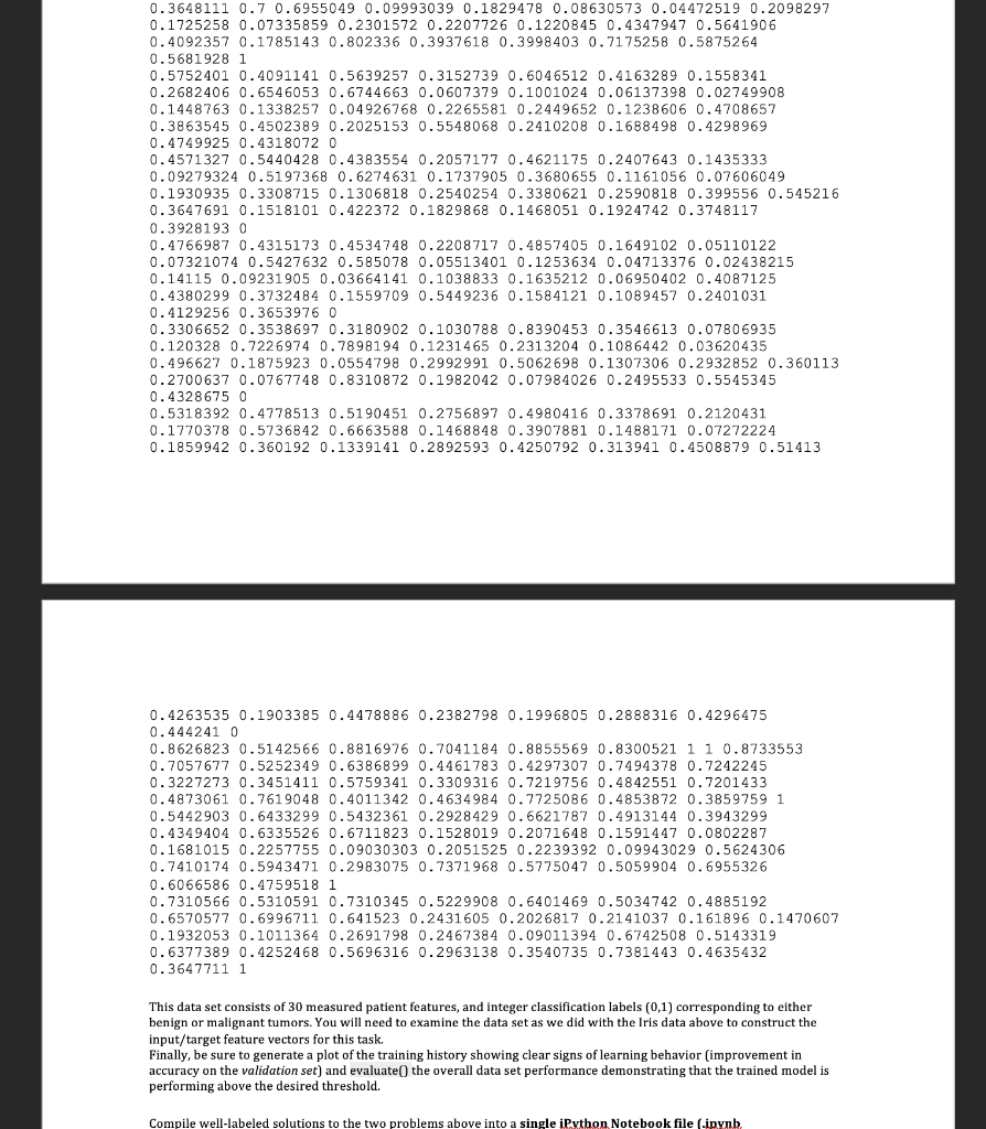
Jupiter Notebook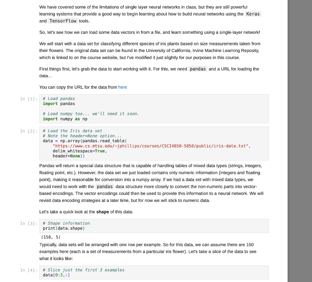

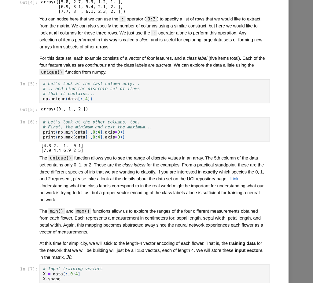
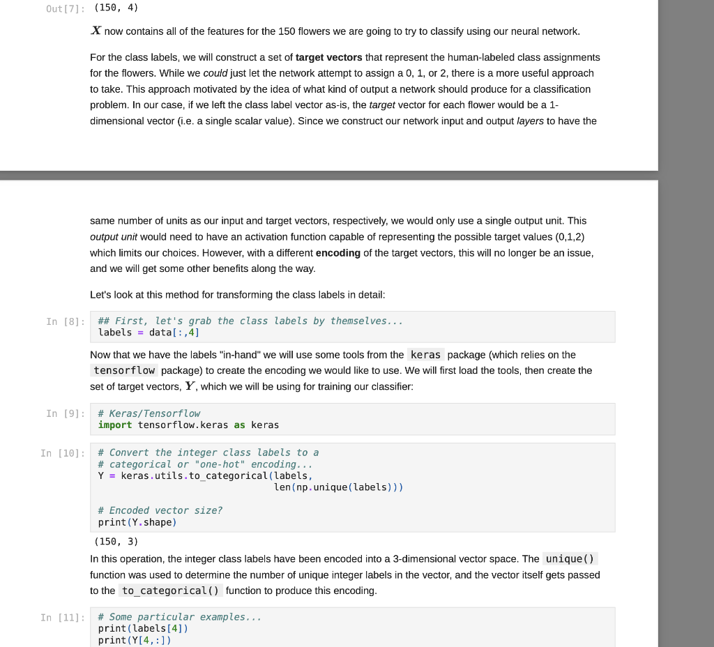
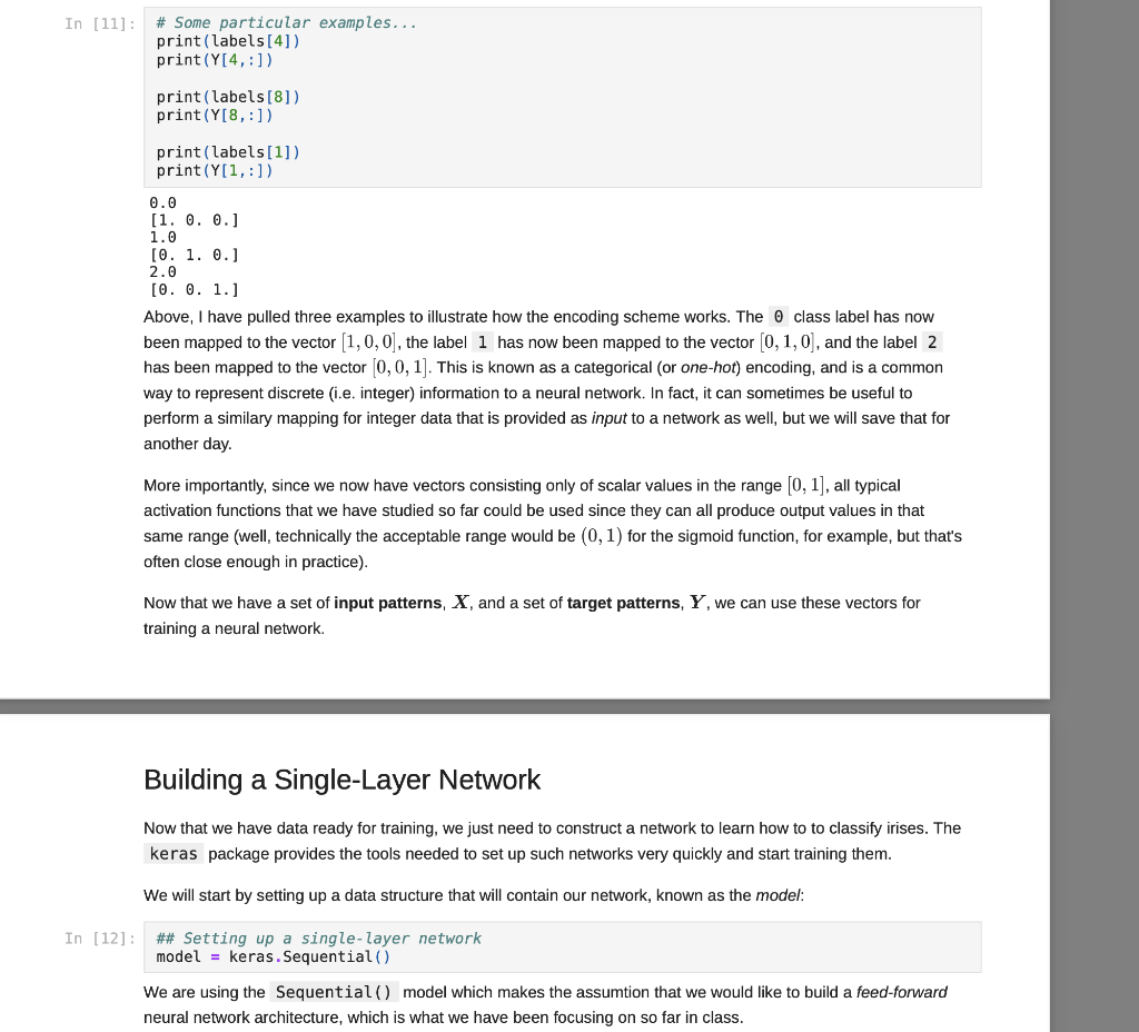
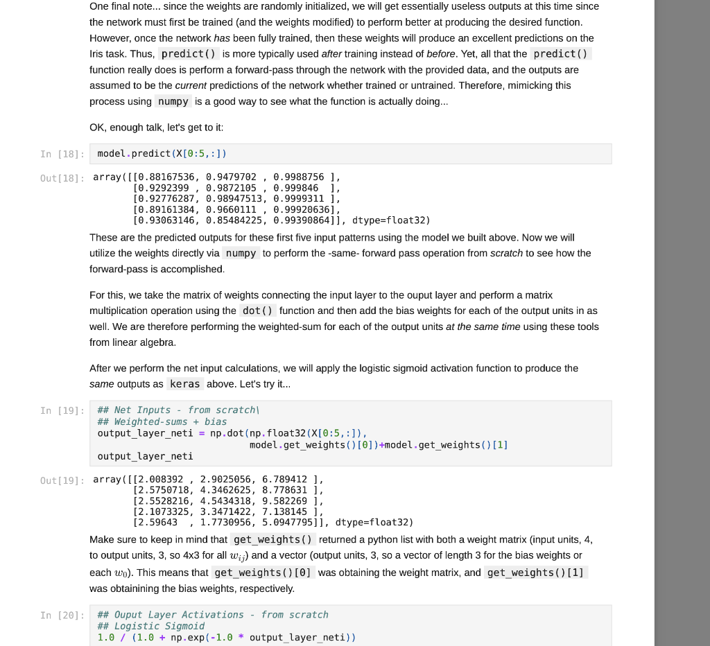
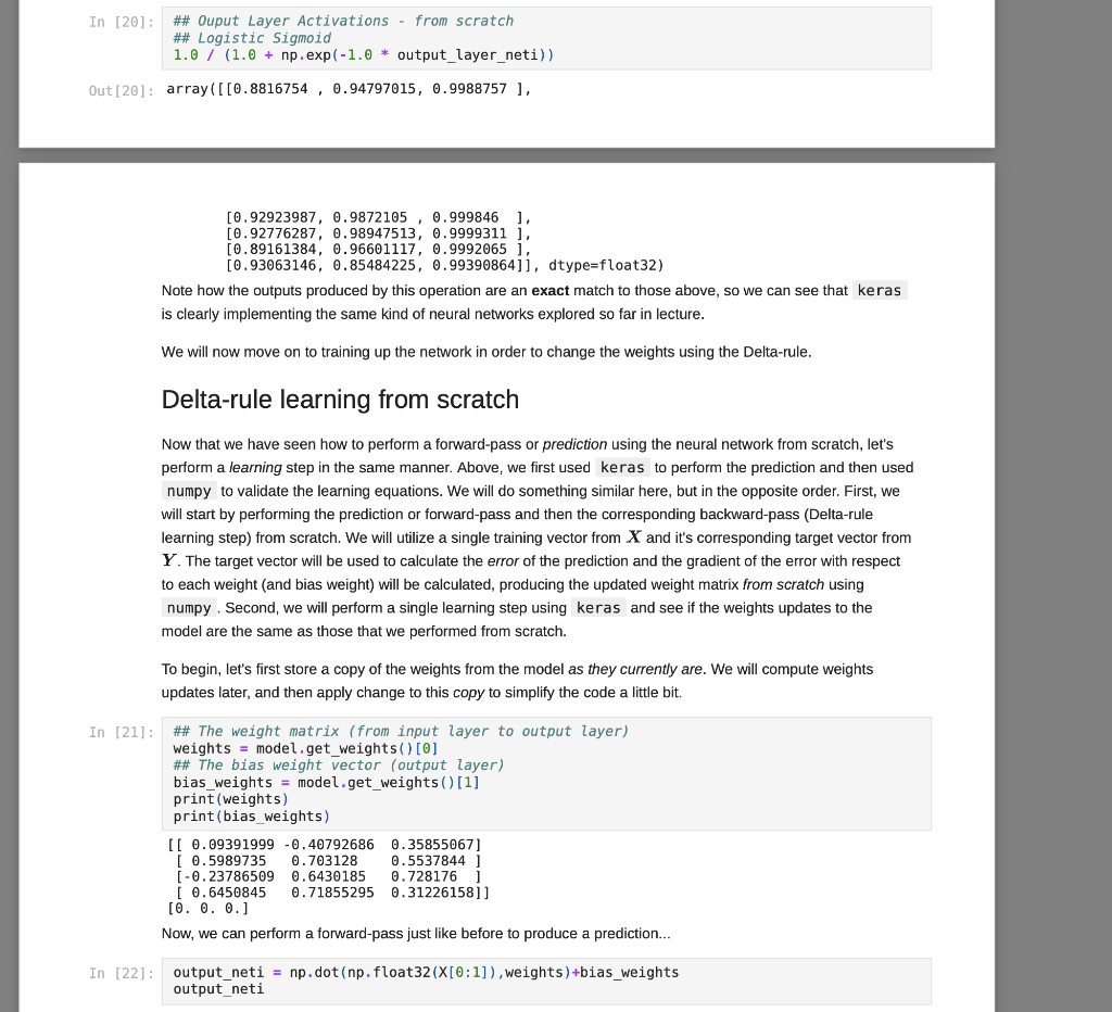
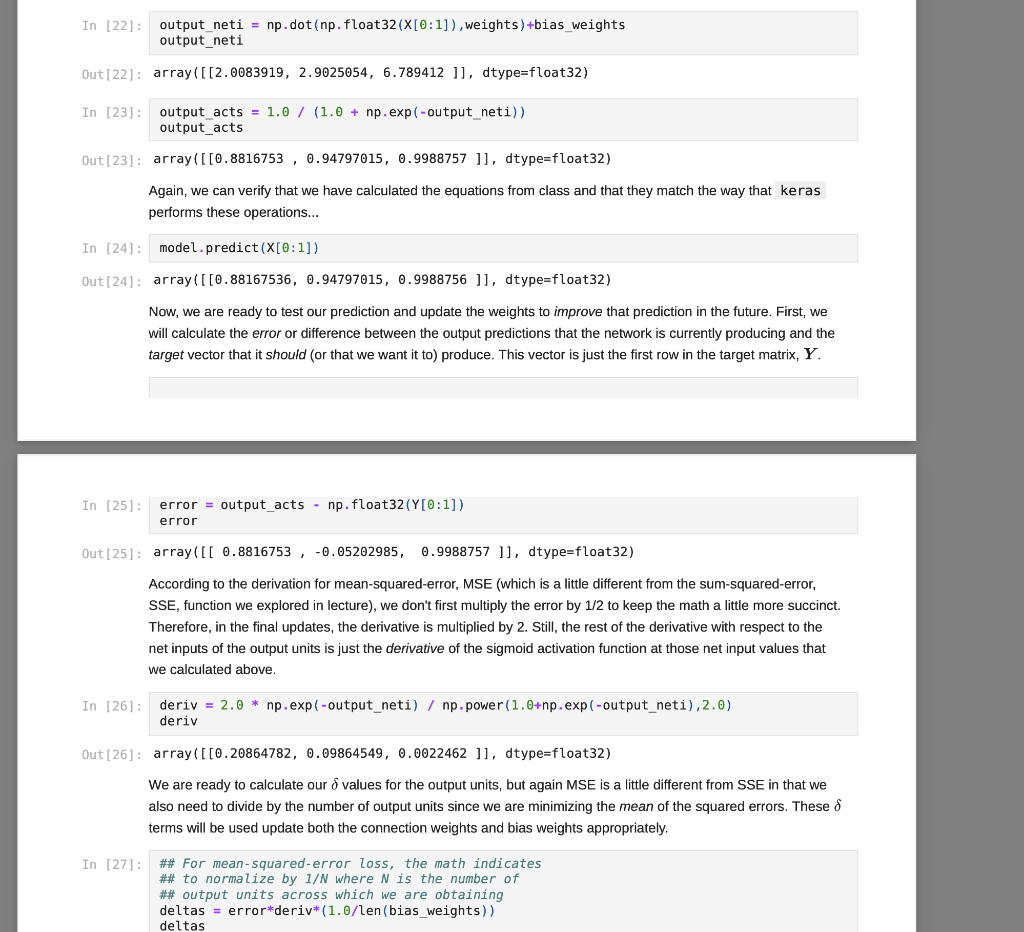
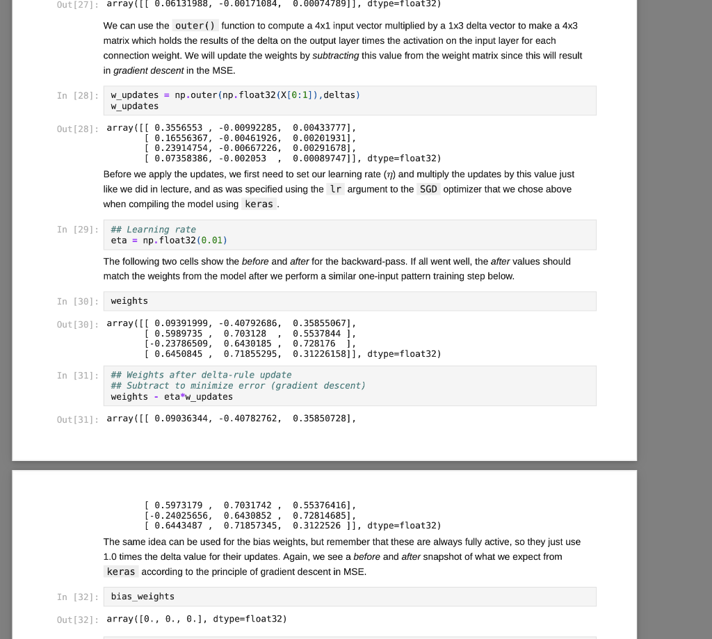
We have covered some of the limitations of single layer neural networks in class, but they are still powerful learning systems that provide a good way to begin learning about how to build neural networks using the Keras and TensorFlow tools. So, let's see how we can load some data vectors in from a file, and learn something using a single-layer network! We will start with a data set for classifying different species of iris plants based on size measurements taken from their flowers. The original data set can be found in the University of California, Irvine Machine Learning Reposity, which is linked to on the course website, but I've modified it just slightly for our purposes in this course. First things first, let's grab the data to start working with it. For this, we need pandas and a URL for loading the data... You can copy the URL for the data from here In [1]: # Load pandas import pandas # Load numpy too... we'll need it soon. import numpy as np In [2] : # Load the Iris data set # Note the header=None option. data = np.array (pandas. read table "https://www.cs.mtsu.edu/-iphillips/courses/CSCI4850-5850/public/iris-data.txt", delim_whitespace=True, header=None)) Pandas will return a special data structure that is capable of handling tables of mixed data types (strings, integers, floating point, etc.). However, the data set we just loaded contains only numeric information integers and floating point), making it reasonable for conversion into a numpy array. If we had a data set with mixed data types, we would need to work with the pandas data structure more closely to convert the non-numeric parts into vector- based encodings. The vector encodings could then be used to provide this information to a neural network. We will revisit data encoding strategies at a later time, but now we will stick to numeric data, Let's take a quick look at the shape of this data: In [3] : # Shape information print (data. shape) (150, 5) Typically, data sets will be arranged with one row per example. So for this data, we can assume there are 150 examples here (each is a set of measurements from a particular iris flower). Let's take a slice of the data to see what it looks like: In [4] : # Slice just the first 3 examples data[0:3,:] Out [4]: array([[5.8, 2.7, 3.9, 1.2, 1. [6.9, 3.1, 5.4, 2.1, 2. ] [7.7, 3.,6.1, 2.3, 2. ]]) You can notice here that we can use the operator ( 0:3 ) to specify a list of rows that we would like to extract from the matrix. We can also specify the number of columns using a similar construct, but here we would like to look at all columns for these three rows. We just use the : operator alone to perform this operation. Any selection of items performed in this way is called a slice, and is useful for exploring large data sets or forming new arrays from subsets of other arrays. For this data set, each example consists of a vector of four features, and a class label (five items total). Each of the four feature values are continuous and the class labels are discrete. We can explore the data a little using the unique() function from numpy. In [5]: # Let's look at the last column only... # .. and find the discrete set of items # that it contains... np.unique (data[:,4]) Out[5]: array([0., 1., 2.1) In [6] : # Let's look at the other columns, too. # First, the minimum and next the maximum... print(np.min(data[:,0:4], axis=0)) print(np.max (data[:,6:4], axis=0)) [4.3 2. 1. 0.1] [7.9 4.4 6.9 2.5] The unique() function allows you to see the range of discrete values in an array. The 5th column of the data set contains only 0, 1, or 2. These are the class labels for the examples. From a practical standpoint, these are the three different species of iris that we are wanting to classify. If you are interested in exactly which species the 0, 1, and 2 represent, please take a look at the details about the data set on the UCI repository page - Link. Understanding what the class labels correspond to in the real world might be important for understanding what our network is trying to tell us, but a proper vector encoding of the class labels alone is sufficient for training a neural network The min() and max() functions allow us to explore the ranges of the four different measurements obtained from each flower. Each represents a measurement in centimeters for: sepal length, sepal width, petal length, and petal width. Again, this mapping becomes abstracted away since the neural network experiences each flower as a vector of measurements. At this time for simplicity, we will stick to the length-4 vector encoding of each flower. That is, the training data for the network that we will be building will just be all 150 vectors, each of length 4. We will store these input vectors in the matrix, X: In [7] : # Input training vectors X = data[:,0:4] X. shape Out[7]: (150, 4) X now contains all of the features for the 150 flowers we are going to try to classify using our neural network. For the class labels, we will construct a set of target vectors that represent the human-labeled class assignments for the flowers. While we could just let the network attempt to assign a 0, 1, or 2, there is a more useful approach to take. This approach motivated by the idea of what kind of output a network should produce for a classification problem. In our case, if we left the class label vector as-is, the target vector for each flower would be a 1- dimensional vector (i.e. a single scalar value). Since we construct our network input and output layers to have the same number of units as our input and target vectors, respectively, we would only use a single output unit. This output unit would need to have an activation function capable of representing the possible target values (0,1,2) which limits our choices. However, with a different encoding of the target vectors, this will no longer be an issue, and we will get some other benefits along the way. Let's look at this method for transforming the class labels in detail: In [8]: ## First, let's grab the class labels by themselves... labels = data[:,4] Now that we have the labels "in-hand" we will use some tools from the keras package (which relies on the tensorflow package) to create the encoding we would like to use. We will first load the tools, then create the set of target vectors, Y, which we will be using for training our classifier: In [9]: # Keras/Tensorflow import tensorflow.keras as keras In [10]: # Convert the integer class labels to a # categorical or "one-hot" encoding... Y = keras.utils.to_categorical(labels, len(np.unique(labels))) # Encoded vector size? print(Y.shape) (150, 3) In this operation, the integer class labels have been encoded into a 3-dimensional vector space. The unique() function was used to determine the number of unique integer labels in the vector, and the vector itself gets passed to the to_categorical() function to produce this encoding. In [11]: # Some particular examples... print(Labels[4]) print (Y[4,:]) In [11]: # Some particular examples... print (labels [4]) print(Y[4,:]) print (labels [8]) print(Y[8,:]) print(labels[1]) print(Y[1,:]) 0.0 [1.0.0.] 1.0 [0. 1. 0.] 2.0 [0. 0. 1.) Above, I have pulled three examples to illustrate how the encoding scheme works. The class label has now been mapped to the vector (1,0,0], the label 1 has now been mapped to the vector (0,1,0, and the label 2 has been mapped to the vector 0, 0, 1). This is known as a categorical (or one-hot) encoding, and is a common way to represent discrete (.e. integer) information to a neural network. In fact, it can sometimes be useful to perform a similary mapping for integer data that is provided as input to a network as well, but we will save that for another day. More importantly, since we now have vectors consisting only of scalar values in the range [0, 1], all typical activation functions that we have studied so far could be used since they can all produce output values in that same range (well, technically the acceptable range would be (0,1) for the sigmoid function, for example, but that's often close enough in practice). Now that we have a set of input patterns, X, and a set of target patterns, Y, we can use these vectors for training a neural network. Building a Single-Layer Network Now that we have data ready for training, we just need to construct a network to learn how to to classify irises. The keras package provides the tools needed to set up such networks very quickly and start training them. We will start by setting up a data structure that will contain our network, known as the model: In [12] : ## Setting up a single-layer network model = keras. Sequential() We are using the Sequential() model which makes the assumtion that we would like to build a feed-forward neural network architecture, which is what we have been focusing on so far in class. Now that we have the container, let's create a single layer network. We do this by adding it to the model using the add() member function. However, we also need to specify the kind of layer we want to add, and some of its details. For our purposes, we are interested in adding a single layer (really, the output layer). Remember, the input layer is rather simple in that it doesn't perform computation, and instead just holds input pattern data during training and prediction (passing data through the network). So, we just need to tell this output layer that it will receive data from the input layer of a certain size. We also need to create all of the connection weights between the input and output layer units, but this is all taken care of for us by the Dense() function. In a nutshell, when making a layer using the Sequential() model, all weights leading into that layer will also need to be specified. There are different ways of connecting layers together, but for now we will mainly focus on densely connected networks, where all units in the previous layer will be connected to all units in the layer we are creating. Again, the Dense() function provides all of the functionality that we need for this operation: In [13] # Add a densely connected layer of units # and specify the input layer size (note, # the input layer is assumed to be there, # which makes this a single-layer network!) # Input size - 4 input_size = X. shape[1] # Output size - 3 output_size = Y.shape[1] # We are using a sigmoid activation # function, AND the input size was # provided within a python list []... model.add(keras.layers.Dense(output_size, activation='sigmoid', input_shape=[input size])) A lovely new neural network! You can use the summary() function to get glimpse into what the Keras tools have created for us: In [14]: model. summary() Model: "sequential" Layer (type) Output Shape Param # dense (Dense) (None, 3) 15 ======== Total params: 15 Trainable params: 15 Non-trainable params: 0 This network follows the conventions we have utilized in class for neural units. That is the neural units, weight matrices, and bias weights have all been created for us using the keras tools. For example, we have a 4x3 weight matrix (12 connection weights), and three output units each with a bias weight, W.. (3 bias weights total). Hence, we have 15 total weights that can be changed during the learning process, and these are known as trainable parameters in the keras framework. The output units utilize the weighted sum calculation we have discussed in class (net input) and we have also specified a sigmoid activation function for output. You can find some additional details about the network's structure by generating and image to display in your notebook: In [15]: keras.utils.plot_model(model, to_file='single_layer_network.png', show_shapes=True, expand_nested=True) Out [15] : dense_input: InputLayer input: [(?, 4)] output: (?, 4)] dense: Dense input: (?, 4) output: (?, 3) You can see that some additional information (like details about the input layer) are provided by this format. You can also see how the layers are connected together (directional arrows), their layer types (eg. Dense), and their input/output shapes. There are two things to keep in mind at this point, and the diagram above illustrates these concepts: 1. The input shape for the Dense layer is (?,4) and the output shape for the Dense layer is (7,3). First of all, each of these shapes indicates that they each are a 2 dimensional tensor (also known as a matrix). Second, the ? is a flexible placeholder for the length of the first dimension of the tensor. The reason for this is because this network is built to accept patterns of length 4, but the network cannot know how many patterns it will be dealing with at any particular moment in time. Remember, we can utilize parallel processing in many ways in neural networks, and one way is to simply have the network process multiple inputs vectors/patterns at the same time (weights are held constant while this entire groups of vectors is propagated through the model). If we wanted to have it operate on a single pattern, we could provide it with an input tensor of shape (1,4) (one pattern on each row, only one row). However, we could pass more patterns into the network at the same time by just adding additional rows of input patterns to the tensor. The ? for all layers is replaced by the number of patterns (the length of the first dimension in the tensor). So, the output from the network would correspondingly be a (1,3) tensor (one pattern produces an output activation vector of length 3 - remember, we have 3 iris species). 2. The weights for the Dense layer are stored internally inside of the Dense layer itself, so the arrow is just showing how the output tensor from the Input layer will be copied/sent downstream to the Dense layer. The Dense layer's input shape is of the corresponding shape to receive it, which is a requirement for a properly structured network. However, the fact that the Dense layer has an input shape of (7,4), and an output shape of (?,3) means it will contain a typical dense layer weight matrix of shape 4x3 and 3 bias weights (for computing net inputs, see above), and then perform a rate encoding using the chose activation function (sigmoid - but note that this is not shown in the diagram). However, the model isn't quite ready to go. At this point, model contains only a template for what we want the network to be. We need to compile() the network to create the tensorflow data structures that actually compute the neural network. Let's do that now: In [16]: # Prep the model for learning- model.compile(loss=keras. losses.mse, optimizer=keras.optimizers. SGD(lr=0.01), metrics=['accuracy']) Remember, learning requires some method for specifying how to update the weights via experience with the training data. We will use the stochastic gradient descent to perform this operation, and we select this by setting optimizer = keras.optimizers. SGD(lr=0.01) (note, the learning rate, lr, setting). However, we need to select an error function as well that we would like to minimize for the optimizer to know what to optimize. In the current literature, since not all functions for describing goodness are really metrics for measuring error, the more general term, loss, is often used. We will be using a loss function that is very similar to the SSE function we studied in class, but here it's the Mean-Squared-Error (loss=keras. losses.mse ). Overall, you can think about this as being similar to multiplying the SSE by some fraction (like we did to derive the delta rule) based on the number of training examples used in each batch for calculating the weight update. Finally, while we will use loss to optimize the weights in the network, a more intuitive metric of performance is added to the model as well: accuracy. While accuracy isn't something used for optimization, if we assume that the strongest ouput from the network (whichever of the three output units produces the highest value) is the network's best guess at what the current iris example should be, then we can calculate the fraction of the iris patterns that it is classifying correctly. Thus, 0.0 accuracy would indicate that the network is classifying -none-of the examples properly, but 1.0 accuracy would indicate that the network is classifying -all- of the examples properly. There are other things that the compile() function takes care of for us, such as setting the weights to some reasonable starting values. For now, we will trust the compile() function to do this job. However, we can buon There are other things that the compile() function takes care of for us, such as setting the weights to some reasonable starting values. For now, we will trust the compile() function to do this job. However, we can always catch a glimpse of what the current weight values are in the network if needed: In [17]: # Examine the bias and connection weights... model.get_weights() Out[17]: [array( [[ 0.09391999, -0.40792686, 0.358550671 [ 0.5989735, 0.703128 0.5537844 ) [-0.23786509, 0.6430185 , 0.728176 ] [ 0.6450845, 0.71855295, 0.31226158]], dtype=float32), array([0., 0., 0.), dtype=float32)] A python list is returned: the first element contains the 4x3 weight matrix, and the second element contains the 3- element vector of output unit bias weights. You can see that the connection weights are initialized to small random values, and the bias weights are initially set to zero. We will explore other methods for initializing the weights in later assignments. How does it work? Before we move on, let's quickly explore how keras calculates values for the network. In other words, let's perform the forward-pass process of the neural network from scratch using numpy. This way, we can see that keras is actually calculating the expressions for single-layer networks just like how we explored them in class. First, keep in mind that the weights above are incorrect (they are random initial values), and will be changed during training below. However, we can still see what the current predictions of the network will be. That is, given some input patterns, X, what would the network output for those examples? The predict() function will allow keras to do this work, and we will choose to perform this operation for the first five patterns in the network. After that, we will explore applying the forward-pass equations by computing them outselves using the same weights above to see how keras computes a forward-pass in just the same was as we have discussed in lecture. So, let's call the predict() function using the first five training patterns. In then end, this function will give us the final activations for the output layer neurons. Since we have a one-hot encoding strategy with three values for our targets, Y, we also asked keras to build the output layer using an equivalent number of neurons. Therefore, if we provide 5 training patterns as input, we will expect the predict() function to return a 5x3 matrix where each row contains the output activations for one of the five patterns. It is easy to process more than one pattern using this function due to the nature of linear algebra operations as we will see below when we compute the same activations from scratch using numpy to implement the forward-pass equations. One final note... since the weights are randomly initialized, we will get essentially useless outputs at this time since the network must first be trained and the weights modified) to perform better at producing the desired function. However, once the network has been fully trained, then these weights will produce an excellent predictions on the Iris task. Thus, predict() is more typically used after training instead of before. Yet, all that the predict() function really does is perform a forward-pass through the network with the provided data, and the outputs are assumed to be the current predictions of the network whether trained or untrained. Therefore, mimicking this process using numpy is a good way to see what the function is actually doing... OK, enough talk, let's get to it: In [18]: model.predict(X[0:5,:]) Out[18]: array([10.88167536, 0.9479702, 0.9988756 ], [0.9292399 0.9872105, 0.999846 ) [0.92776287, 0.98947513, 0.9999311 ], [0.89161384, 0.9660111, 0.99920636), [0.93063146, 0.85484225, 0.99390864]], dtype=float32) These are the predicted outputs for these first five input patterns using the model we built above. Now we will utilize the weights directly via numpy to perform the -same-forward pass operation from scratch to see how the forward-pass is accomplished. For this, we take the matrix of weights connecting the input layer to the ouput layer and perform a matrix multiplication operation using the dot() function and then add the bias weights for each of the output units in as well. We are therefore performing the weighted-sum for each of the output units at the same time using these tools from linear algebra. After we perform the net input calculations, we will apply the logistic sigmoid activation function to produce the same outputs as keras above. Let's try it... In [19]: ## Net Inputs from scratchi ## Weighted-sums + bias output_layer_neti = np.dot (np. float32(X[0:5,:]). model.get_weights()[])+model.get_weights() [1] output_layer_neti Out[19]: array([[2.008392 , 2.9025056, 6.789412 ], [2.5750718, 4.3462625, 8.778631 ), [2.5528216, 4.5434318, 9.582269 ], [2.1073325, 3.3471422, 7.138145 ], [2.59643 1 1.7730956, 5.0947795j, dtype=float32) Make sure to keep in mind that get_weights() returned a python list with both a weight matrix (input units, 4, to output units, 3, so 4x3 for all wij) and a vector (output units, 3, so a vector of length 3 for the bias weights or each wo). This means that get_weights() [0] was obtaining the weight matrix, and get_weights() [1] was obtainining the bias weights, respectively. In [20]: ## Ouput Layer Activations - from scratch ## Logistic Sigmoid 1.0 / (1.0 + np.exp(-1.0 * output_layer_neti)) In [20]: ## Ouput Layer Activations - from scratch ## Logistic Sigmoid 1.0 / (1.0 + np.exp(-1.0 * output_layer_neti)) Out[20]: array([[0.8816754, 0.94797015, 0.9988757 ], [0.92923987, 0.9872105 0.999846 1. [0.92776287, 0.98947513, 0.9999311 ], [0.89161384, 0.96601117, 0.9992065 ], [0.93063146, 0.85484225, 0.99390864]], dtype=float32) Note how the outputs produced by this operation are an exact match to those above, so we can see that keras is clearly implementing the same kind of neural networks explored so far in lecture. We will now move on to training up the network in order to change the weights using the Delta-rule. Delta-rule learning from scratch Now that we have seen how to perform a forward-pass or prediction using the neural network from scratch, let's perform a learning step in the same manner. Above, we first used keras to perform the prediction and then used numpy to validate the learning equations. We will do something similar here, but in the opposite order. First, we will start by performing the prediction or forward-pass and then the corresponding backward-pass (Delta-rule learning step) from scratch. We will utilize a single training vector from X and it's corresponding target vector from Y. The target vector will be used to calculate the error of the prediction and the gradient of the error with respect to each weight (and bias weight) will be calculated producing the updated weight matrix from scratch using numpy. Second, we will perform a single learning step using keras and see if the weights updates to the model are the same as those that we performed from scratch. To begin, let's first store a copy of the weights from the model as they currently are. We will compute weights updates later, and then apply change to this copy to simplify the code a little bit. In [21]: ## The weight matrix (from input layer to output layer) weights = model.get_weights() [O] ## The bias weight vector (output layer) bias_weights = model.get_weights() [1] print (weights) print(bias_weights) [[ 0.09391999 -0.40792686 0.35855067] [ 0.5989735 0.703128 0.5537844 [-0.23786509 0.6430185 0.728176 ] [ 0.6450845 0.71855295 0.31226158]] [0.0.0.] Now, we can perform a forward-pass just like before to produce a prediction... In [22]: output_neti = np.dot(np. float32(X[0:1]), weights) +bias_weights output neti In [22]: output_neti = np.dot(np. float32(X[0:1]), weights) +bias_weights output_neti Out[22]: array([[2.0083919, 2.9025054, 6.789412 ]], dtype=float32) In [23]: output_acts = 1.0 / (1.0 + np.exp(-output_neti)) output_acts Out [23]: array ( [[0.8816753, 0.94797015, 0.9988757 ]], dtype=float32) Again, we can verify that we have calculated the equations from class and that they match the way that keras performs these operations... In [24]: model.predict(X[0:1]) Out [24]: array([[0.88167536, 0.94797015, 0.9988756 ]], dtype=float32) Now, we are ready to test our prediction and update the weights to improve that prediction in the future. First, we will calculate the error or difference between the output predictions that the network is currently producing and the target vector that it should (or that we want it to) produce. This vector is just the first row in the target matrix, Y. In [25]: error = output_acts - np.float32(Y[0:1]) error Out [25]: array([[ 0.8816753, -0.05202985, 0.9988757 ]], dtype=float32) According to the derivation for mean-squared-error, MSE (which is a little different from the sum-squared-error, SSE, function we explored in lecture), we don't first multiply the error by 1/2 to keep the math a little more succinct. Therefore, in the final updates, the derivative is multiplied by 2. Still, the rest of the derivative with respect to the net inputs of the output units is just the derivative of the sigmoid activation function at those net input values that we calculated above. In [26]: deriv = 2.0 * np.exp(-output_neti) / np. power(1.0+np.exp(-output_neti),2.0) deriv Out [26]: array([[0.20864782, 0.09864549, 0.0022462 ]], dtype=float32) We are ready to calculate our & values for the output units, but again MSE is a little different from SSE in that we also need to divide by the number of output units since we are minimizing the mean of the squared errors. These 8 terms will be used update both the connection weights and bias weights appropriately. In [27]: ## For mean-squared-error loss, the math indicates ## to normalize by 1/N where N is the number of ## output units across which we are obtaining deltas = error*deriv*(1.0/len (bias_weights)) deltas Out[27]: array([[ 0.06131988, -0.00171084, 0.00074789]], dtype=float32) We can use the outer() function to compute a 4x1 input vector multiplied by a 1x3 delta vector to make a 4x3 matrix which holds the results of the delta on the output layer times the activation on the input layer for each connection weight. We will update the weights by subtracting this value from the weight matrix since this will result in gradient descent in the MSE. In [28]: w_updates = np.outer(np. float32(X[0:1]), deltas) W_updates Out [28]: array([[ 0.3556553 -0.00992285, 0.00433777), [ 0.16556367, -0.00461926, 0.00201931) 0.23914754, -0.00667226, 0.00291678], [ 0.07358386, -0.002053 0.00089747]], dtype=float32) Before we apply the updates, we first need to set our learning rate (n) and multiply the updates by this value just like we did in lecture, and as was specified using the Ir argument to the SGD optimizer that we chose above when compiling the model using keras. In [29]: ## Learning rate eta = np.float32(0.01) The following two cells show the before and after for the backward-pass. If all went well, the after values should match the weights from the model after we perform a similar one-input pattern training step below. In [30]: weights Out [30]: array([[ 0.09391999, -0.40792686, 0.35855067] [ 0.5989735, 0.703128 0.5537844 ) [-0.23786509, 0.6430185, 0.728176 ], [ 0.6450845, 0.71855295, 0.31226158]], dtype=float32) In [31]: ## Weights after delta-rule update ## Subtract to minimize error (gradient descent) weights - eta*w_updates Out (31): array([[ 0.09036344, -0.40782762, 0.35850728), [ 0.5973179, 0.7031742, 0.55376416) [ -0.24025656, 0.6430852 0.728146851 [ 0.6443487, 0.71857345, 0.3122526 l], dtype=float32) The same idea can be used for the bias weights, but remember that these are always fully active, so they just use 1.0 times the delta value for their updates. Again, we see before and after snapshot of what we expect from keras according to the principle of gradient descent in MSE. In [32]: bias_weights Out[32]: array([0., 0., 0.], dtype=float32) In [32] : bias_weights Out[32]: array([0., 0., 0.), dtype=float32) In [33] : ## Bias weights after delta-rule update ## Subtract to minimize error (gradient descent) bias_weights - eta*deltas Out[33]: array([[-6.1319879e-04, 1.7108367e-05, -7.47892008-06]], dtype=float32) We're ready to validate our approach and see if keras produces the same result as our calculated weight updates above. Let's ask keras to perform a single epoch of training on a data set with a single input-target pair. Each epoch is a complete pass through the training data, and the batch size determines how many pattern gradients will be summed together before performing the weight update (to produce a smoother descent in error, use larger batch sizes). However, we are just testing our model here, so we will just do a single pass on one pattern, so it makes sense to set the batch size to 1 (it would ignore any larger number anyway since there isn't more training data provided) Now for the moment of truth... In [34] history = model.fit(X[0:1],Y[0:1], batch_size=1, epochs=1, verbose=0) model.get_weights() Out [34]: (array([[ 0.09036344, -0.40782762, 0.35850728] [ 0.5973179, 0.7031742, 0.55376416) [-0.24025656, 0.6430852, 0.72814685) [ 0.6443487 0.71857345, 0.3122526 ]], dtype=float32), array([-6.1319885e-04, 1.7108367e-05, -7.4790328e-06], dtype=float32)] Notice that we performed the weight update to our model using the fit() function. This is the training function provided by keras for adapting weights in our neural networks, and we will see how to use it in a more general way below. However, after this single forward-backward pass, we can now print the new weights from the model, and you can see that they are now a nearly exact match to our calculated weights updates using numpy (some small rouding errors on the weights will be within an acceptable tolerance for floating point operations such as these - different approximations are used to improve performance across different libraries). Therefore, in principle we could design our networks from scratch in this way all of the time. However, you can clearly now appreciate how simple the keras framework makes performing these operations. This is especially true when you need an architecture that combines many different types of layers and other options that we will explore in the future. Now that we at least understand in principle how these nets are computing their results, let's see how we might use them to learn something about the Iris data set. Training a Single-Layer Network Time to get training! First, select a batch size for the stochastic gradient update: the number of patterns experienced between weight updates. Second, choose the number of epochs (complete passes through the data) that you would like to peform. Third, select a certain fraction of the data that you would like to use for validation of Training a Single-Layer Network Time to get training! First, select a batch size for the stochastic gradient update: the number of patterns experienced between weight updates. Second, choose the number of epochs (complete passes through the data) that you would like to peform. Third, select a certain fraction of the data that you would like to use for validation of your training results (0.5 would mean that 50% of the data is not used for training, but instead used to test for generalization). We will utilize the fit() member function of our model for perfoming the training, which accepts these three options to control its behavior: In [35]: # Basic training parameters batch size = 16 epochs = 10 validation_split = 0.5 ==== # Train the model and record the training # history for later examination history = model. fit(X, Y, batch size = batch size, epochs = epochs, verbose = 1, validation_split = validation_split) Epoch 1/10 5/5 [=========== ========== - Os 42ms/step - loss: 0.5805 - accuracy: 0.3333 - val_ loss: 0.5731 val_accuracy: 0.3333 Epoch 2/10 5/5 [========= =] - Os 7ms/step - loss: 0.5737 - accuracy: 0.3333 - val_l OSS: 0.5652 val_accuracy: 0.3333 Epoch 3/10 5/5 (===== Os 7ms/step loss: 0.5659 - accuracy: 0.3333 - val_1 OSS: 0.5562 val_accuracy: 0.3333 Epoch 4/10 5/5 (======= Os 7ms/step loss: 0.5569 - accuracy: 0.3333 - val_1 OSS: 0.5456 - val_accuracy: 0.3333 Epoch 5/10 5/5 (====== ==============] - Os 8ms/step - loss: 0.5464 - accuracy: 0.3333 - val_1 OSS: 0.5338 val_accuracy: 0.3333 Epoch 6/10 5/5 (======== - Os 8ms/step - loss: 0.5344 - accuracy: 0.3333 - val_l OSS: 0.5202 val_accuracy: 0.3333 Epoch 7/10 5/5 (======= Os 8ms/step loss: 0.5211 - accuracy: 0.3333 - val_1 oss: 0.5055 - val_accuracy: 0.3333 Epoch 8/10 5/5 [========= ============] . Os 7ms/step loss: 0.5063 . accuracy: 0.3333 - val_1 OSS: 0.4896 val accuracy: 0.3333 # Train the model and record the training # history for later examination history = model. fit(X, Y, batch_size = batch_size, epochs = epochs, verbose = 1, validation_split = validation_split) Epoch 1/10 5/5 (========= ===========] - Os 42ms/step - loss: 0.5805 - accuracy: 0.3333 - val_ loss: 0.5731 val_accuracy: 0.3333 Epoch 2/10 5/5 [======= ===========] - Os 7ms/step - loss: 0.5737 - accuracy: 0.3333 - val_1 oss: 0.5652 - val_accuracy: 0.3333 Epoch 3/10 5/5 (===== ========] - Os 7ms/step - loss: 0.5659 - accuracy: 0.3333 - val_1 oss: 0.5562 - val_accuracy: 0.3333 Epoch 4/10 5/5 (======== - Os 7ms/step - loss: 0.5569 - accuracy: 0.3333 - val_1 oss: 0.5456 - val_accuracy: 0.3333 Epoch 5/10 5/5 (========== ===========] - Os 8ms/step - loss: 0.5464 - accuracy: 0.3333 - val_1 OSS: 0.5338 - val_accuracy: 0.3333 Epoch 6/10 5/5 [======== ==============] - Os 8ms/step - loss: 0.5344 accuracy: 0.3333 - val_1 OSS: 0.5202 - val_accuracy: 6.3333 Epoch 7/10 5/5 [====== ===========] - Os Sms/step - loss: 0.5211 - accuracy: 0.3333 - val_l oss: 0.5055 val_accuracy: 0.3333 Epoch 8/10 5/5 (====== ==========] - Os 7ms/step - loss: 0.5063 - accuracy: 0.3333 - val_1 oss: 0.4896 - val_accuracy: 0.3333 Epoch 9/10 5/5 (====== - Os 7ms/step - loss: 0.4906 - accuracy: 0.3333 - val_l oss: 0.4734 val_accuracy: 0.3333 Epoch 10/10 5/5 [========= =============] - Os Sms/step - loss: 0.4748 - accuracy: 0.3333 - val_l OSS: 0.4580 - val_accuracy: 0.3333 Notice that you will get some output for each epoch that you train the network, indicating progress through the training. You can turn off this output by using the verbose=0 option at any time. This is sometimes useful since there are other ways that we can look at the training performance using the history data that came back from the fitting process. You can see that the loss values were decreasing (error was going down), even if accuracy wasn't necessarily increasing. To make this network perform better we could: 1) Increase the number epochs used in the training process 2) Increase the learning rate on the stochastic gradient optimizer 3) Rebuild the network starting from our model = keras. Sequential() statement to initialize the weights at a better starting location in the weight space. 3) Other things that we will explore at a later time (don't use any other tricks for this assignment... Let's plot the history information for a moment to see what happened across training. This is just a graphical depiction of what happened during the training process: In [36]; import matplotlib.pyplot as plt matplotlib inline plt.figure(1) # summarize history for accuracy plt. subplot(211) plt.plot(history.history['accuracy']) plt.plot(history.history['val_accuracy']) plt.title('model accuracy') plt.ylabel('accuracy' plt.xlabel('epoch') plt.legend (['train', 'val'), loc=' upper left') # summarize history for loss plt. subplot(212) plt.plot(history.history['loss']) plt.plot(history.history['val_loss']) plt.title('model loss') plt.ylabel('loss') plt.xlabel('epoch') plt.legend (['train', 'val'], loc='upper left') plt. tight_layout() plt.show() model accuracy 0.35 0.34 train val ccuracy 0.33 0.32 0 2 6 8 4 epoch model loss 0.55 train val 0.50 0 2 6 8 epoch These graphical reports (after using verbose=0 ) will be very useful for completing this assignment. Use the code above as a template for constructing your graphs. Limited changes should be needed to complete this Show the bookmarks in this folder assignment. However, let's see how our network performs now on the entire data set. (This is not the best way to assess performance: we should use a testing data set with examples that the network has never seen and that we have never used to tune our hyperparameters. So, the evaluation below is a biased performance evaluation. However, these are small data sets so there isn't much data available for doing this kind of analysis currently: we will use proper techniques in future assignments.) Now that we have trained the network, we can use the evaluate() method to determine this information: plt.figure(1) # summarize history for accuracy plt. subplot(211) plt.plot(history.history['accuracy']) plt.plot(history.history['val_accuracy']) plt.title('model accuracy') plt.ylabel('accuracy' plt.xlabel('epoch') plt.legend (['train', 'val'), loc=' upper left') # summarize history for loss plt. subplot(212) plt.plot(history.history['loss']) plt.plot(history.history['val_loss']) plt.title('model loss') plt.ylabel('loss') plt.xlabel('epoch') plt.legend (['train', 'val'], loc='upper left') plt. tight_layout() plt.show() model accuracy 0.35 0.34 train val ccuracy 0.33 0.32 0 2 6 8 4 epoch model loss 0.55 train val 0.50 0 2 6 8 epoch These graphical reports (after using verbose=0 ) will be very useful for completing this assignment. Use the code above as a template for constructing your graphs. Limited changes should be needed to complete this Show the bookmarks in this folder assignment. However, let's see how our network performs now on the entire data set. (This is not the best way to assess performance: we should use a testing data set with examples that the network has never seen and that we have never used to tune our hyperparameters. So, the evaluation below is a biased performance evaluation. However, these are small data sets so there isn't much data available for doing this kind of analysis currently: we will use proper techniques in future assignments.) Now that we have trained the network, we can use the evaluate() method to determine this information: These graphical reports (after using verbose=6 ) will be very useful for completing this assignment. Use the code above as a template for constructing your graphs. Limited changes should be needed to complete this assignment. However, let's see how our network performs now on the entire data set. (This is not the best way to assess performance: we should use a testing data set with examples that the network has never seen and that we have never used to tune our hyperparameters. So, the evaluation below is a biased performance evaluation. However, these are small data sets so there isn't much data available for doing this kind of analysis currently: we will use proper techniques in future assignments.) Now that we have trained the network, we can use the evaluate() method to determine this information: In [37]: score = model. evaluate (X, Y, verbose=1) print('Test loss:', score[0]) print('Test accuracy: score[1]) 5/5 [=========== ======] - Os lms/step - loss: 0.4617 - accuracy: 0.3333 Test Loss: 0.4617256820201874 Test accuracy: 0.3333333432674408 In the end, we are only getting 33% of the validation examples classified correctly! However, we can use one or more) of the three suggested tricks above for improving the performance of the network. Unless you rebuild the model again from scratch, training can be carried over from previous fit() operations. So, if we ran fit() again now for another 10 epochs, it would be 20 epochs total of training. However, the history information from the previous 10 epochs may be lost, so be sure to keep records of the training process or restart from scratch if Show the bookmarks in this folder you want to train for more epochs from the very beginning Some models also take a long time to evaluate, so the verbose() option is available to help determine how long this process takes to complete, but feel free to turn it off by setting it to zero. If you want to get a fresh model with new initial weights and no experience with the problem (sometimes needed due to optimization errors or bad hyperparameter choices in your models), then you will need to rerun all model construction/compilation steps: start back at model = keras. Sequential(). This will ensure that you get a freshly constructed model for subsequent training/validation and ensure that any hyperparameter changes have These graphical reports (after using verbose=6 ) will be very useful for completing this assignment. Use the code above as a template for constructing your graphs. Limited changes should be needed to complete this assignment. However, let's see how our network performs now on the entire data set. (This is not the best way to assess performance: we should use a testing data set with examples that the network has never seen and that we have never used to tune our hyperparameters. So, the evaluation below is a biased performance evaluation. However, these are small data sets so there isn't much data available for doing this kind of analysis currently: we will use proper techniques in future assignments.) Now that we have trained the network, we can use the evaluate() method to determine this information: In [37]: score = model. evaluate (X, Y, verbose=1) print('Test loss:', score[0]) print('Test accuracy: score[1]) 5/5 [=========== ======] - Os lms/step - loss: 0.4617 - accuracy: 0.3333 Test Loss: 0.4617256820201874 Test accuracy: 0.3333333432674408 In the end, we are only getting 33% of the validation examples classified correctly! However, we can use one or more) of the three suggested tricks above for improving the performance of the network. Unless you rebuild the model again from scratch, training can be carried over from previous fit() operations. So, if we ran fit() again now for another 10 epochs, it would be 20 epochs total of training. However, the history information from the previous 10 epochs may be lost, so be sure to keep records of the training process or restart from scratch if Show the bookmarks in this folder you want to train for more epochs from the very beginning Some models also take a long time to evaluate, so the verbose() option is available to help determine how long this process takes to complete, but feel free to turn it off by setting it to zero. If you want to get a fresh model with new initial weights and no experience with the problem (sometimes needed due to optimization errors or bad hyperparameter choices in your models), then you will need to rerun all model construction/compilation steps: start back at model = keras. Sequential(). This will ensure that you get a freshly constructed model for subsequent training/validation and ensure that any hyperparameter changes have Assignment Now that you know how to build single-layer networks and train them, you will need to explore training them on some existing data sets, and evaluating their performance. 1. Utilize the methods learned in the tutorial above to train a good single layer network for the Iris data set (>95% accuracy). You must the data set from below 5.8 2.7 3.9 1.2 1 6.9 3.1 5.4 2.1 2 7.7 3.0 6.1 2.3 2 5.7 3.0 4.2 1.2 1 5.1 3.7 1.5 0.4 0 5.6 2.9 3.6 1.3 1 6.2 2.9 4.3 1.3 1 5.0 3.2 1.2 0.2 0 6.7 3.0 5.0 1.7 1 6.4 2.8 5.6 2.2 2 6.3 3.3 6.0 2.5 2 6.3 3.4 5.6 2.4 2 6.7 3.1 4.4 1.4 1 4.6 3.2 1.4 0.20 4.4 2.9 1.4 0.2 0 6.0 3.4 4.5 1.6 1 5.4 3.0 4.5 1.5 1 6.3 2.9 5.6 1.8 2 4.4 3.2 1.3 0.2 0 5.4 3.4 1.7 0.2 0 6.4 3.2 4.5 1.5 1 7.7 2.6 6.9 2.3 2 5.8 2.7 5.1 1.9 2 4.9 3.1 1.5 0.2 0 4.8 3.0 1.4 0.1 0 7.1 3.0 5.9 2.1 2 7.9 3.8 6.4 2.0 2 5.1 3.8 1.6 0.2 0 5.5 4.2 1.4 0.20 5.9 3.0 4.2 1.5 1 4.9 3.1 1.5 0.1 0 5.3 3.7 1.5 0.2 0 5.2 3.4 1.4 0.2 0 6.0 2.9 4.5 1.5 1 5.7 2.6 3.5 1.0 1 7.2 3.6 6.1 2.5 2 6.8 3.2 5.9 2.3 2 7.7 3.8 6.7 2.2 2 6.7 3.3 5.7 2.5 2 Subtitle 5.2 3.5 1.5 0.2 0 5.1 3.5 1.4 0.3 0 6.9 3.1 4.9 1.5 l 6.5 3.2 5.1 2.0 2 6.8 2.8 4.8 1.4 1 7.0 3.2 4.7 1.4 1 6.2 2.2 4.5 1.5 1 4.8 3.1 1.6 0.20 6.0 2.2 4.0 1.0 1 6.6 2.9 4.6 1.3 1 5.1 3.8 1.5 0.3 0 5.7 2.8 4.5 1.3 1 6.4 2.9 4.3 1.3 1 5.6 3.0 4.5 1.5 i 7.2 3.0 5.8 1.6 2 6.5 3.0 5.5 1.8 2 5.5 2.6 4.4 1.2 1 6.2 2.8 4.8 1.8 2 5.4 3.9 1.7 0.4 0 6.0 2.7 5.1 1.6 1 5.6 3.0 4.1 1.3 1 6.8 3.0 5.5 2.1 2 6.5 2.8 4.6 1.5 1 6.9 3.2 5.7 2.3 2 5.0 3.3 1.4 0.2 0 5.0 2.0 3.5 1.0 i 5.8 2.6 4.0 1.2 1 7.2 3.2 6.0 1.8 2 6.7 3.1 5.6 2.4 2 4.9 3.0 1.4 0.2 0 5.4 3.4 1.5 0.4 0 6.1 2.9 4.7 1.4 1 6.3 2.8 5.1 1.5 2 7.3 2.9 6.3 1.8 2 6.3 2.3 4.4 1.3 1 4.8 3.4 1.9 0.2 0 4.3 3.0 1.1 0.1 0 6.7 3.0 5.2 2.3 2 5.0 3.6 1.4 0.2 0 5.7 4.4 1.5 0.4 0 5.1 2.5 3.0 1.11 5.6 2.7 4.2 1.3 1 6.1 3.0 4.6 1.4 1 5.1 3.3 1.7 0.5 0 4.9 2.5 4.5 1.72 6.0 2.2 5.0 1.5 2 6.4 3.1 5.5 1.8 2 6.3 2.5 4.9 1.5 1 Be sure to generate a plot of the training history that shows improvement in the validation accuracy (starts low and grows high), and also evaluate() the performance on the complete data set as shown above demonstrating that the trained model is performing above the desired threshold. 2. Utilize the methods learned in the above tutorial to train a good single-layer classifier (>90% accuracy) for the Wisconsin (Diagnostic) Breast Cancer data set. You must use this data set below 0.6766275 0.6260183 0.6472149 0.4302279 0.5525704 0.3491604 0.343955 0.4110835 0.6424342 0.5776888 0.1912635 0.1358444 0.13899 0.1063261 0.1243816 0.1360414 0.09368687 0.2273158 0.248765 0.1118298 0.681465 0.6138474 0.6086783 0.3815233 0.5610961 0.3030246 0.4596645 0.6721649 0.5959626 0.4476145 1 0.5186766 0.5481161 0.5167639 0.2578169 0.6450428 0.5408222 0.33388 0.4365308 0.7407895 0.7105911 0.08858336 0.2012692 0.09599636 0.03882331 0.1430132 0.2256278 0.06770202 0.2561091 0.1841672 0.1243633 0.4889012 0.6703674 0.4872611 0.2108369 0.6850854 0.6278828 0.4424121 0.9281787 0.6423622 0.6144578 1 0.5190324 0.5773931 0.5113528 0.2627349 0.5185435 0.3850608 0.2410965 0.1856859 0.4782895 0.6308498 0.07845458 0.2268168 0.1011829 0.03603836 0.1362673 0.3426145 0.1661111 0.3042243 0.2074731 0.1476542 0.4295228 0.5504643 0.4215764 0.172426 0.4609164 0.2997164 0.292492 0.3797251 0.3401627 0.3857349 0 0.4087513 0.3714358 0.3925199 0.1618952 0.6401469 0.2382166 0.1243674 0.09786282 0.5851974 0.6746716 0.07079708 0.2386899 0.07129208 0.02644781 0.1592355 0.15613 0.1049495 0.1522637 0.2334389 0.1211126 0.3440622 0.442067 0.3265924 0.1099201 0.6073675 0.1899811 0.2073482 0.2553608 0.4430551 0.4424096 0 0.3728211 0.5056008 0.3539523 0.135026 0.6548348 0.172872 0.1131912 0.1525845 0.5713816 0.6609195 0.1294466 0.5346981 0.1145132 0.04282553 0.5152586 0.1023634 0.04709596 0.214624 0.4402787 0.1193029 0.318535 0.594671 0.2933121 0.09468735 0.680593 0.09697543 0.09432907 0.2314777 0.4343176 0.3733976 O 0.3842049 0.5595723 0.3649337 0.1439024 0.5386169 0.166271 0.08467666 0.06978131 0.6631579 0.6134031 0.1071006 0.3318321 0.1019108 0.03725563 0.2101831 0.1586411 0.0755303 0.1979542 0.2335655 0.09014745 0.3540511 0.6467501 0.3331608 0.1150682 0.5853549 0.1603025 0.1539137 0.2572165 0.4466707 0.369253 0 0.530772 0.3800916 0.5116711 0.2746501 0.4955936 0.2475101 0.1297798 0.1600895 0.5549342 0.5817939 0.08513749 0.08872057 0.08307552 0.04299152 0.1050755 0.1307238 0.05833333 0.1591021 0.1454085 0.0797252 0.4766926 0.3677836 0.4458599 0.2131171 0.4784367 0.2637996 0.2516773 0.3941581 0.4049412 0.3986988 0 0.8256848 0.686609 0.8143236 0.6677329 0.5819461 0.4869716 0.4568885 0.6148111 0.6279605 0.6474754 0.3682562 0.1972364 0.3297088 0.2873478 0.2064889 0.2114476 0.1135606 0.3250616 0.2013933 0.1023123 0.8604329 0.6966088 0.8200637 0.6920545 0.665319 0.3899811 0.4648562 0.8910653 0.4674601 0.4181687 1 0.4027037 0.6894094 0.3806897 0.1582167 0.4212362 0.1103937 0.03826148 0.01553181 0.6148026 0.5775862 0.04211625 0.1827431 0.04818016 0.01587053 0.1173466 0.1216396 0.04123737 0.05919682 0.1946802 0.06876676 0.3351831 0.6812677 0.3177548 0.1063235 0.4134322 0.1353497 0.08698083 0.07158076 0.4291955 0.3415422 0 0.4699395 0.6428208 0.4461538 0.215074 0.5380049 0.1506948 0.06494845 0.1027833 0.5325658 0.5730706 0.07253742 0.2763562 0.05978162 0.03242346 0.1852875 0.05968981 0.03813131 0.1222012 0.1706143 0.06126005 0.3981687 0.6909568 0.3634156 0.1487776 0.5790656 0.1004726 0.1110224 0.2063574 0.3681832 0.3271325 0 0.3158307 0.3943483 0.301008 0.09636146 0.5075275 0.222872 0.1106139 0.11834 0.6348684 0.6794951 0.1872955 0.2456499 0.194586 0.05566212 0.3511083 0.2141064 0.08116162 0.2852813 0.3593414 0.1398794 0.2769423 0.357287 0.2598328 0.07099201 0.4559748 0.1179584 0.07540735 0.1636426 0.3666767 0.3581205 0 0.3648111 0.7 0.6955049 0.09993039 0.1829478 0.08630573 0.04472519 0.2098297 0.1725258 0.07335859 0.2301572 0.2207726 0.1220845 0.4347947 0.5641906 0.4092357 0.1785143 0.802336 0.3937618 0.3998403 0.7175258 0.5875264 0.5681928 1 0.5752401 0.4091141 0.5639257 0.3152739 0.6046512 0.4163289 0.1558341 0.2682406 0.6546053 0.6744663 0.0607379 0.1001024 0.06137398 0.02749908 0.1448763 0.1338257 0.04926768 0.2265581 0.2449652 0.1238606 0.4708657 0.3863545 0.4502389 0.2025153 0.5548068 0.2410208 0.1688498 0.4298969 0.4749925 0.4318072 0 0.4571327 0.5440428 0.4383554 0.2057177 0.4621175 0.2407643 0.1435333 0.09279324 0.5197368 0.6274631 0.1737905 0.3680655 0.1161056 0.07606049 0.1930935 0.3308715 0.1306818 0.2540254 0.3380621 0.2590818 0.399556 0.545216 0.3647691 0.1518101 0.422372 0.1829868 0.1468051 0.1924742 0.3748117 0.3928193 0 0.4766987 0.4315173 0.4534748 0.2208717 0.4857405 0.1649102 0.05110122 0.07321074 0.5427632 0.585078 0.05513401 0.1253634 0.04713376 0.02438215 0.14115 0.09231905 0.03664141 0.1038833 0.1635212 0.06950402 0.4087125 0.4380299 0.3732484 0.1559709 0.5449236 0.1584121 0.1089457 0.2401031 0.4129256 0.3653976 O 0.3306652 0.3538697 0.3180902 0.1030788 0.8390453 0.3546613 0.07806935 0.120328 0.7226974 0.7898194 0.1231465 0.2313204 0.1086442 0.03620435 0.496627 0.1875923 0.0554798 0.2992991 0.5062698 0.1307306 0.2932852 0.360113 0.2700637 0.0767748 0.8310872 0.1982042 0.07984026 0.2495533 0.5545345 0.4328675 0 0.5318392 0.4778513 0.5190451 0.2756897 0.4980416 0.3378691 0.2120431 0.1770378 0.5736842 0.6663588 0.1468848 0.3907881 0.1488171 0.07272224 0.1859942 0.360192 0.1339141 0.2892593 0.4250792 0.313941 0.4508879 0.51413 0.4263535 0.1903385 0.4478886 0.2382798 0.1996805 0.2888316 0.4296475 0.444241 0 0.8626823 0.5142566 0.8816976 0.7041184 0.8855569 0.8300521 11 0.8733553 0.7057677 0.5252349 0.6386899 0.4461783 0.4297307 0.7494378 0.7242245 0.3227273 0.3451411 0.5759341 0.3309316 0.7219756 0.4842551 0.7201433 0.4873061 0.761 9048 0.4011342 0.4634984 0.7725086 0.4853872 0.3859759 1 0.5442903 0.6433299 0.5432361 0.2928429 0.6621787 0.4913144 0.3943299 0.4349404 0.6335526 0.6711823 0.1528019 0.2071648 0.1591447 0.0802287 0.1681015 0.2257755 0.09030303 0.2051525 0.2239392 0.09943029 0.5624306 0.7410174 0.5943471 0.2983075 0.7371968 0.5775047 0.5059904 0.6955326 0.6066586 0.4759518 1 0.7310566 0.5310591 0.7310345 0.5229908 0.6401469 0.5034742 0.4885192 0.6570577 0.6996711 0.641523 0.2431605 0.2026817 0.2141037 0.161896 0.1470607 0.1932053 0.1011364 0.2691798 0.2467384 0.09011394 0.6742508 0.5143319 0.6377389 0.4252468 0.5696316 0.2963138 0.3540735 0.7381443 0.4635432 0.3647711 1 This data set consists of 30 measured patient features, and integer classification labels (0,1) corresponding to either benign or malignant tumors. You will need to examine the data set as we did with the Iris data above to construct the input/target feature vectors for this task. Finally, be sure to generate a plot of the training history showing clear signs of learning behavior (improvement in accuracy on the validation set) and evaluate the overall data set performance demonstrating that the trained model is performing above the desired threshold. Compile well-labeled solutions to the two problems above into a single iPython Notebook file idynb. 2. Utilize the methods learned in the above tutorial to train a good single-layer classifier (>90% accuracy) for the Wisconsin (Diagnostic) Breast Cancer data set. You must use this data set below 0.6766275 0.6260183 0.6472149 0.4302279 0.5525704 0.3491604 0.343955 0.4110835 0.6424342 0.5776888 0.1912635 0.1358444 0.13899 0.1063261 0.1243816 0.1360414 0.09368687 0.2273158 0.248765 0.1118298 0.681465 0.6138474 0.6086783 0.3815233 0.5610961 0.3030246 0.4596645 0.6721649 0.5959626 0.4476145 1 0.5186766 0.5481161 0.5167639 0.2578169 0.6450428 0.5408222 0.33388 0.4365308 0.7407895 0.7105911 0.08858336 0.2012692 0.09599636 0.03882331 0.1430132 0.2256278 0.06770202 0.2561091 0.1841672 0.1243633 0.4889012 0.6703674 0.4872611 0.2108369 0.6850854 0.6278828 0.4424121 0.9281787 0.6423622 0.6144578 1 0.5190324 0.5773931 0.5113528 0.2627349 0.5185435 0.3850608 0.2410965 0.1856859 0.4782895 0.6308498 0.07845458 0.2268168 0.1011829 0.03603836 0.1362673 0.3426145 0.1661111 0.3042243 0.2074731 0.1476542 0.4295228 0.5504643 0.4215764 0.172426 0.4609164 0.2997164 0.292492 0.3797251 0.3401627 0.3857349 0 0.4087513 0.3714358 0.3925199 0.1618952 0.6401469 0.2382166 0.1243674 0.09786282 0.5851974 0.6746716 0.07079708 0.2386899 0.07129208 0.02644781 0.1592355 0.15613 0.1049495 0.1522637 0.2334389 0.1211126 0.3440622 0.442067 0.3265924 0.1099201 0.6073675 0.1899811 0.2073482 0.2553608 0.4430551 0.4424096 0 0.3728211 0.5056008 0.3539523 0.135026 0.6548348 0.172872 0.1131912 0.1525845 0.5713816 0.6609195 0.1294466 0.5346981 0.1145132 0.04282553 0.5152586 0.1023634 0.04709596 0.214624 0.4402787 0.1193029 0.318535 0.594671 0.2933121 0.09468735 0.680593 0.09697543 0.09432907 0.2314777 0.4343176 0.3733976 0 0.3842049 0.5595723 0.3649337 0.1439024 0.5386169 0.166271 0.08467666 0.06978131 0.6631579 0.6134031 0.1071006 0.3318321 0.1019108 0.03725563 0.2101831 0.1586411 0.0755303 0.1979542 0.2335655 0.09014745 0.3540511 0.6467501 0.3331608 0.1150682 0.5853549 0.1603025 0.1539137 0.2572165 0.4466707 0.369253 0 0.5208111 0.3879837 0.5080637 0.2606557 0.6927785 0.3876665 0.2335052 0.3510934 0.6960526 0.6512726 0.1780369 0.150911 0.1735214 0.07886389 0.1769354 0.3258493 0.1120202 0.3074446 0.3074098 0.1622319 0.4533851 0.3681873 0.4355096 0.1889046 0.5736748 0.291966 0.2079872 0.4800687 0.4746912 0.4083373 O This data set consists of 30 measured patient features, and integer classification labels (0,1) corresponding to either benign or malignant tumors. You will need to examine the data set as we did with the Iris data above to construct the input/target feature vectors for this task. Finally, be sure to generate a plot of the training history showing clear signs of learning behavior (improvement in accuracy on the validation set) and evaluate(the overall data set performance demonstrating that the trained model is performing above the desired threshold. Compile well-labeled solutions to the two problems above into a single iPython Notebook file (.ipynh 0.472074 0.3757637 0.4495491 0.2205918 0.4501224 0.1463521 0.07640581 0.1316103 0.4559211 0.5457718 0.1412113 0.2360287 0.1228844 0.06704168 0.1439447 0.07666174 0.03429293 0.2049631 0.1354022 0.04808981 0.4539401 0.4511506 0.4160032 0.1952515 0.4519317 0.1170132 0.1078275 0.3439863 We have covered some of the limitations of single layer neural networks in class, but they are still powerful learning systems that provide a good way to begin learning about how to build neural networks using the Keras and TensorFlow tools. So, let's see how we can load some data vectors in from a file, and learn something using a single-layer network! We will start with a data set for classifying different species of iris plants based on size measurements taken from their flowers. The original data set can be found in the University of California, Irvine Machine Learning Reposity, which is linked to on the course website, but I've modified it just slightly for our purposes in this course. First things first, let's grab the data to start working with it. For this, we need pandas and a URL for loading the data... You can copy the URL for the data from here In [1]: # Load pandas import pandas # Load numpy too... we'll need it soon. import numpy as np In [2] : # Load the Iris data set # Note the header=None option. data = np.array (pandas. read table "https://www.cs.mtsu.edu/-iphillips/courses/CSCI4850-5850/public/iris-data.txt", delim_whitespace=True, header=None)) Pandas will return a special data structure that is capable of handling tables of mixed data types (strings, integers, floating point, etc.). However, the data set we just loaded contains only numeric information integers and floating point), making it reasonable for conversion into a numpy array. If we had a data set with mixed data types, we would need to work with the pandas data structure more closely to convert the non-numeric parts into vector- based encodings. The vector encodings could then be used to provide this information to a neural network. We will revisit data encoding strategies at a later time, but now we will stick to numeric data, Let's take a quick look at the shape of this data: In [3] : # Shape information print (data. shape) (150, 5) Typically, data sets will be arranged with one row per example. So for this data, we can assume there are 150 examples here (each is a set of measurements from a particular iris flower). Let's take a slice of the data to see what it looks like: In [4] : # Slice just the first 3 examples data[0:3,:] Out [4]: array([[5.8, 2.7, 3.9, 1.2, 1. [6.9, 3.1, 5.4, 2.1, 2. ] [7.7, 3.,6.1, 2.3, 2. ]]) You can notice here that we can use the operator ( 0:3 ) to specify a list of rows that we would like to extract from the matrix. We can also specify the number of columns using a similar construct, but here we would like to look at all columns for these three rows. We just use the : operator alone to perform this operation. Any selection of items performed in this way is called a slice, and is useful for exploring large data sets or forming new arrays from subsets of other arrays. For this data set, each example consists of a vector of four features, and a class label (five items total). Each of the four feature values are continuous and the class labels are discrete. We can explore the data a little using the unique() function from numpy. In [5]: # Let's look at the last column only... # .. and find the discrete set of items # that it contains... np.unique (data[:,4]) Out[5]: array([0., 1., 2.1) In [6] : # Let's look at the other columns, too. # First, the minimum and next the maximum... print(np.min(data[:,0:4], axis=0)) print(np.max (data[:,6:4], axis=0)) [4.3 2. 1. 0.1] [7.9 4.4 6.9 2.5] The unique() function allows you to see the range of discrete values in an array. The 5th column of the data set contains only 0, 1, or 2. These are the class labels for the examples. From a practical standpoint, these are the three different species of iris that we are wanting to classify. If you are interested in exactly which species the 0, 1, and 2 represent, please take a look at the details about the data set on the UCI repository page - Link. Understanding what the class labels correspond to in the real world might be important for understanding what our network is trying to tell us, but a proper vector encoding of the class labels alone is sufficient for training a neural network The min() and max() functions allow us to explore the ranges of the four different measurements obtained from each flower. Each represents a measurement in centimeters for: sepal length, sepal width, petal length, and petal width. Again, this mapping becomes abstracted away since the neural network experiences each flower as a vector of measurements. At this time for simplicity, we will stick to the length-4 vector encoding of each flower. That is, the training data for the network that we will be building will just be all 150 vectors, each of length 4. We will store these input vectors in the matrix, X: In [7] : # Input training vectors X = data[:,0:4] X. shape Out[7]: (150, 4) X now contains all of the features for the 150 flowers we are going to try to classify using our neural network. For the class labels, we will construct a set of target vectors that represent the human-labeled class assignments for the flowers. While we could just let the network