Answered step by step
Verified Expert Solution
Link Copied!

Question

1 Approved Answer

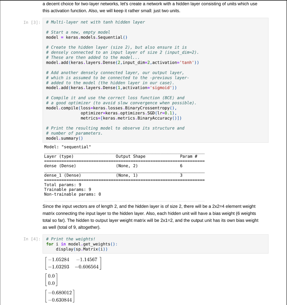
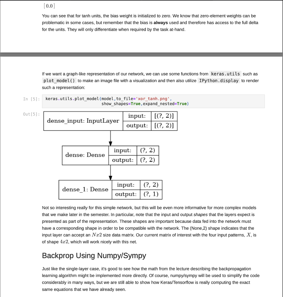
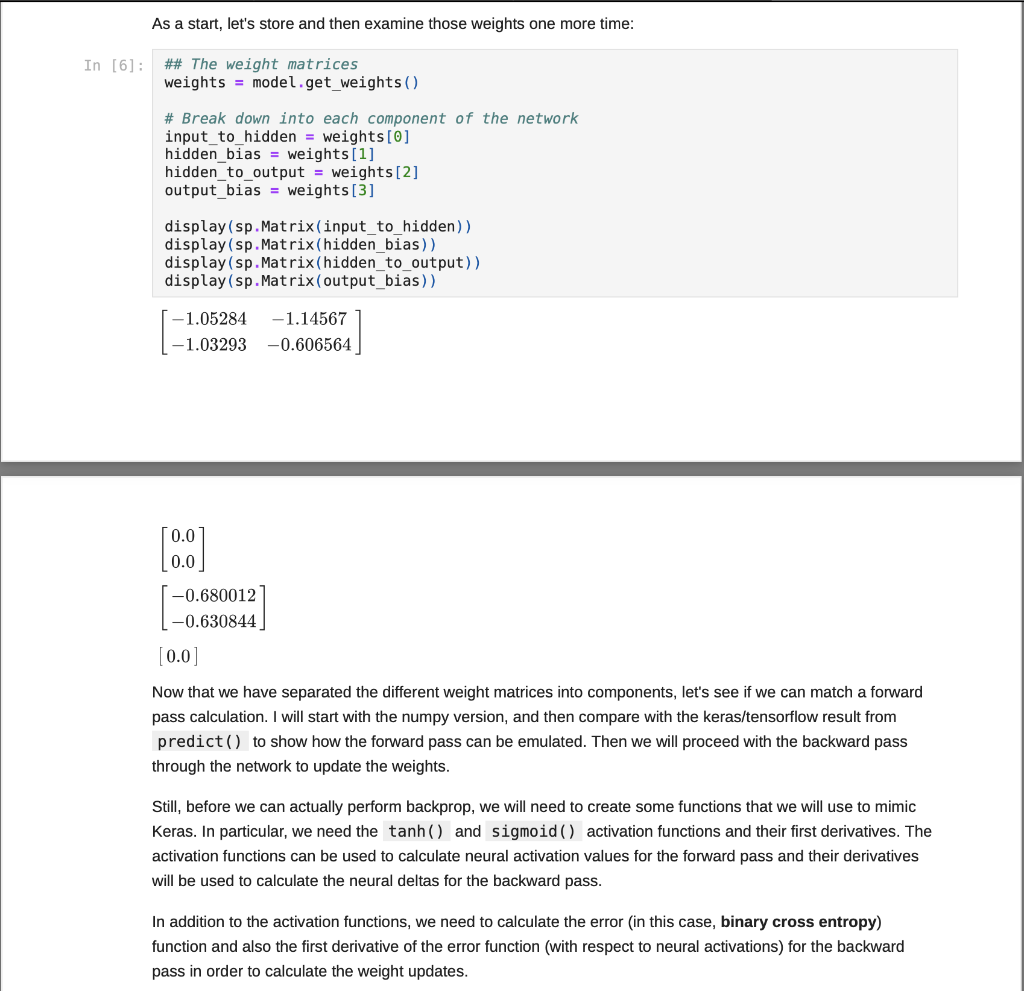
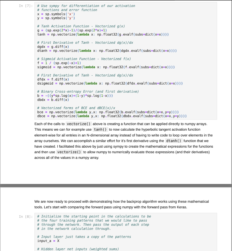
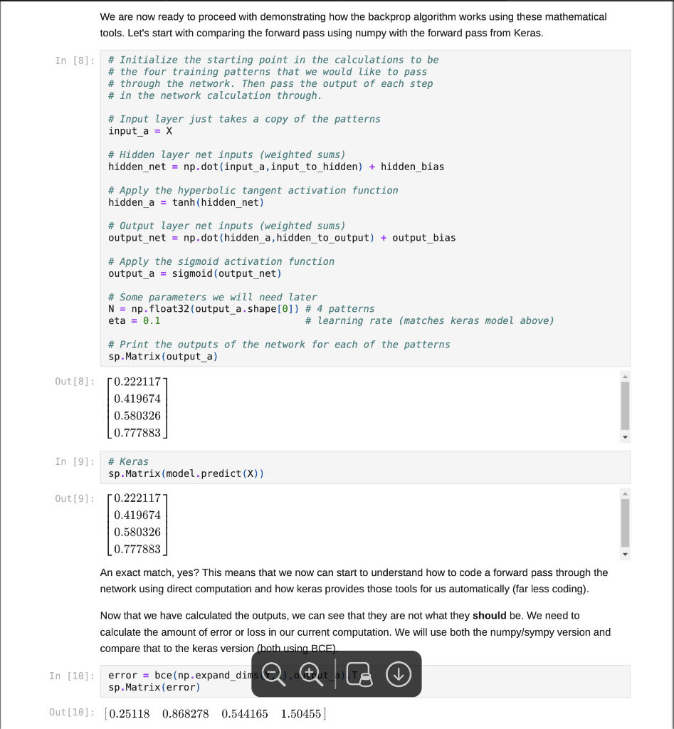
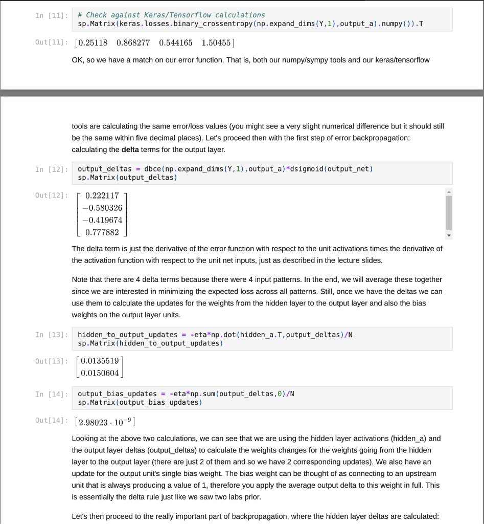
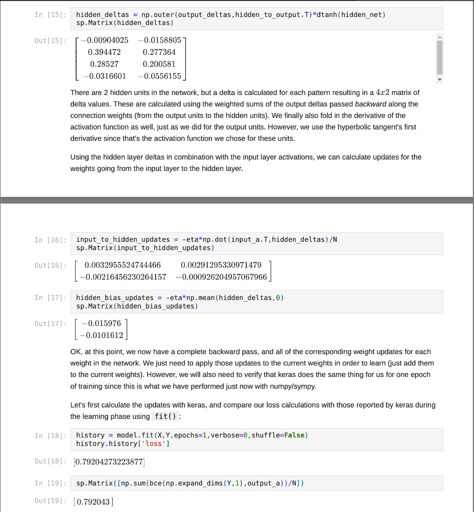
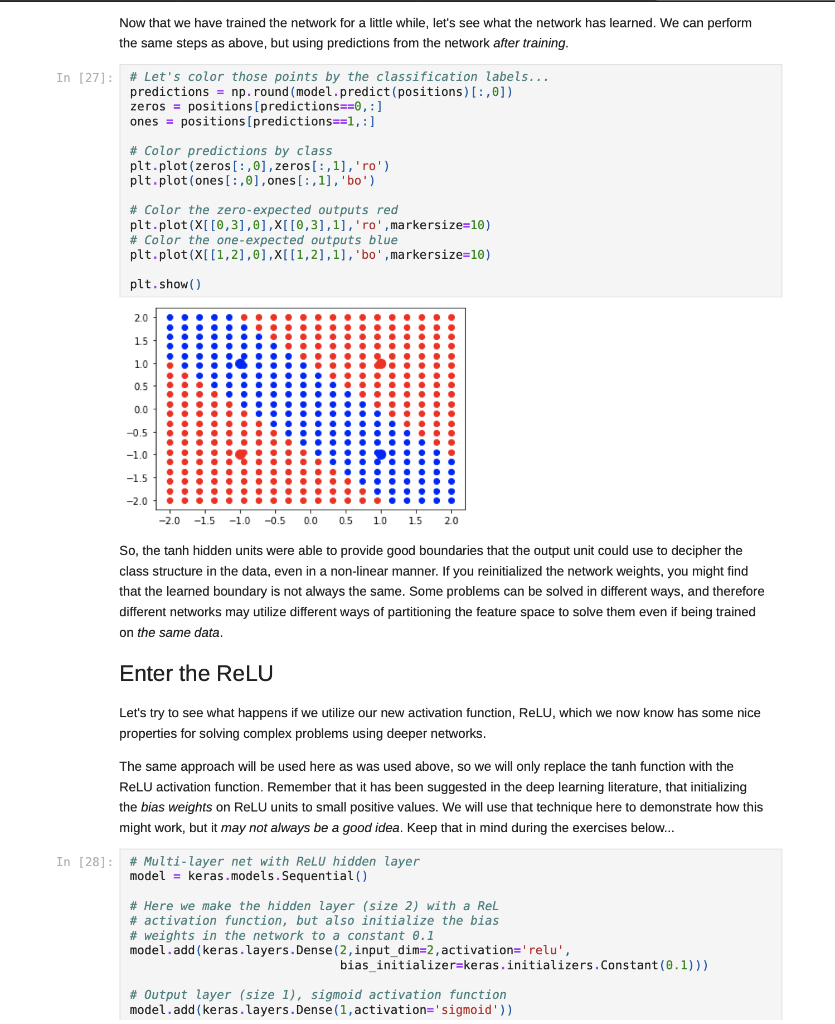
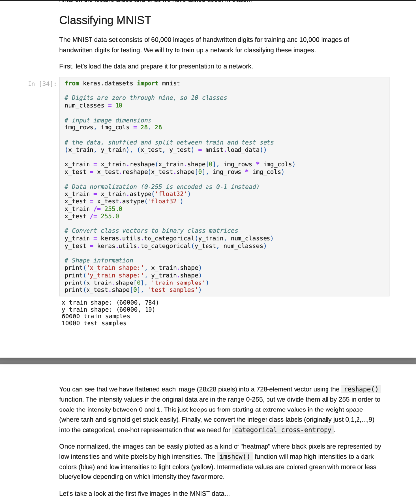
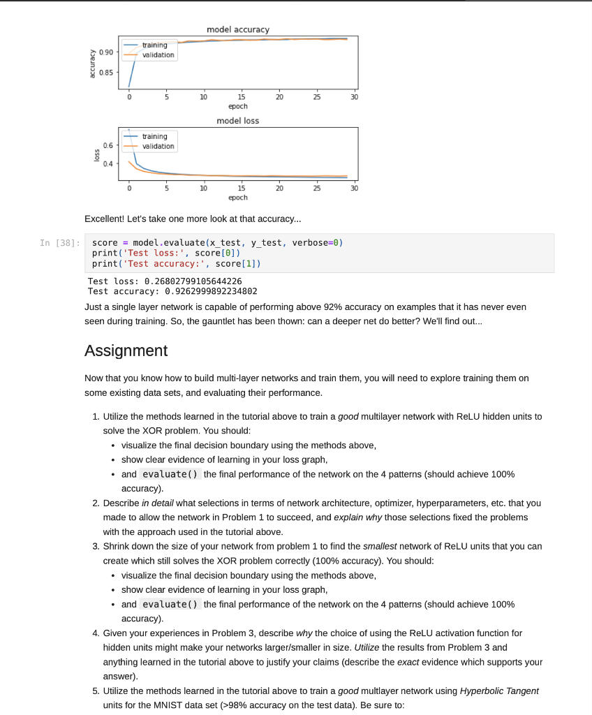
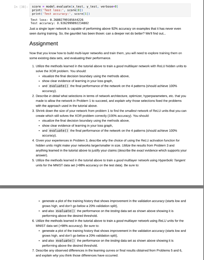
Jupyter Notebook Now that we have tried our hand at some single-layer nets, let's see how they stack up compared to multi-layer nets. :) We

Jupyter Notebookimage text in transcribedimage text in transcribedimage text in transcribedimage text in transcribedimage text in transcribedimage text in transcribedimage text in transcribedimage text in transcribedimage text in transcribedimage text in transcribedimage text in transcribedimage text in transcribedimage text in transcribedimage text in transcribedimage text in transcribedimage text in transcribedimage text in transcribedimage text in transcribedimage text in transcribedimage text in transcribedimage text in transcribedimage text in transcribed

Now that we have tried our hand at some single-layer nets, let's see how they stack up compared to multi-layer nets. :) We will be exploring the basic concepts of learning non-linear functions using the classic XOR problem, and then explore the basics of "deep learning" technology on this problem as well. After that, we will see if a multi-layer approach can perform better than single-layer approach on some data sets that we have seen before. In particular, we will try to explore the wider vs. deeper issue, and see if ReLU really helps. For now, let's look into the XOR problem, and see what insights we can gain when comparing single- and multi- layer network approaches. In [1]: # NN - Tools import numpy as np import tensorflow.keras as keras # Printing from IPython.display import display import sympy as sp sp.init_printing (use_latex=True) # Plotting import matplotlib.pyplot as plt %matplotlib inline Let's create the XOR data set. As we mentioned in class, avoiding zeros in the input patterns is a good general approach for stable learning behavior. In [2]: # XOR data set X = np.array([[-1,-1],[-1,1],[1,-1],[1,1]]) display (sp.Matrix(x)) Y = np.array([0,1,1,0]) display(sp.Matrix(Y)) 1 1 1 0 We are performing a classification task since there are two discrete targets, so using binary cross-entropy error at the output layer makes sense. Also, binary cross-entropy suggest the sigmoid activation function for the output unit since it is comparing only two classes. Given that the hyperbolic tangent (tanh) activation function is a decent choice for two-layer networks, let's create a network with a hidden layer consisting of units which use this activation function. Also, we will keep it rather small: just two units. In [3]: # Multi-Zayer net with tanh hidden Layer # Start a new, empty model model = keras.models. Sequential() # Create the hidden Layer (size 2), but also ensure it is # densely connected to an input layer of size 2 (input_dim=2). # These are then added to the model... model.add(keras.layers.Dense(2, input_dim=2, activation='tanh')) # Add another densely connected layer, our output layer, # which is assumed to be connected to the previous Layer- # added to the model (the hidden Layer in our case). model.add(keras.layers. Dense(1, activation='sigmoid)) # Compile it and use the correct loss function (BCE) and # a good optimizer (to avoid slow convergence when possible). model.compile(loss=keras. losses. BinaryCrossentropy(), optimizer=keras. optimizers. SGD(lr=0.1), metrics=[keras.metrics. BinaryAccuracy (1) # Print the resulting model to observe its structure and # number of parameters. model. summary() Model: "sequential" Layer (type) Output Shape Param # dense (Dense) (None, 2) 6 ======== ======== (None, 1) 3 dense_1 (Dense) ========== Total params: 9 Trainable params: 9 Non-trainable params: 0 Since the input vectors are of length 2, and the hidden layer is of size 2, there will be a 2x2=4 element weight matrix connecting the input layer to the hidden layer. Also, each hidden unit will have a bias weight 6 weights total so far). The hidden to output layer weight matrix will be 2x1=2, and the output unit has its own bias weight as well (total of 9, altogether). In [4]: # Print the weights! for i in model.get_weights(): display (sp. Matrix(i)) 1.05284 -1.14567 -1.03293 -0.606564 0.0 -0.680012 -0.630844 [0.0) You can see that for tanh units, the bias weight is initialized to zero. We know that zero-element weights can be problematic in some cases, but remember that the bias is always used and therefore has access to the full delta for the units. They will only differentiate when required by the task at-hand. If we want a graph-like representation of our network, we can use some functions from keras.utils such as plot_model() to make an image file with a visualization and then also utilize IPython.display to render such a representation: In [5]: keras.utils.plot_model(model, to_file='xor_tanh.png', show_shapes=True, expand_nested=True) Out[5]: dense_input: InputLayer input: [(?, 2)] output: [(?, 2)] dense: Dense input: (?, 2) output: (?, 2) dense_1: Dense input: (?, 2) output: (?, 1) Not so interesting really for this simple network, but this will be even more informative for more complex models that we make later in the semester. In particular, note that the input and output shapes that the layers expect is presented as part of the representation. These shapes are important because data fed into the network must have a corresponding shape in order to be compatible with the network. The (None 2) shape indicates that the input layer can accept an Nx2 size data matrix. Our current matrix of interest with the four input patterns, X, is of shape 4x2, which will work nicely with this net. Backprop Using Numpy/Sympy Just like the single-layer case, it's good to see how the math from the lecture describing the backpropagation learning algorithm might be implemented more directly. Of course, numpy/sympy will be used to simplify the code considerably in many ways, but we are still able to show how Keras/Tensorflow is really computing the exact same equations that we have already seen. As a start, let's store and then examine those weights one more time: In [6]: ## The weight matrices weights = model.get_weights() # Break down into each component of the network input_to_hidden = weights[0] hidden_bias = weights[1] hidden_to_output = weights [2] output_bias = weights [3] display (sp.Matrix(input_to_hidden)) display (sp.Matrix(hidden bias)) display (sp.Matrix(hidden_to_output)) display (sp.Matrix(output_bias)) -1.05284 -1.03293 -1.14567 -0.606564 0.01 0.0 -0.680012 -0.630844 [0.0] Now that we have separated the different weight matrices into components, let's see if we can match a forward pass calculation. I will start with the numpy version, and then compare with the keras/tensorflow result from predict() to show how the forward pass can be emulated. Then we will proceed with the backward pass through the network to update the weights. Still, before we can actually perform backprop, we will need to create some functions that we will use to mimic Keras. In particular, we need the tanh() and sigmoid() activation functions and their first derivatives. The activation functions can be used to calculate neural activation values for the forward pass and their derivatives will be used to calculate the neural deltas for the backward pass. In addition to the activation functions, we need to calculate the error (in this case, binary cross entropy) function and also the first derivative of the error function (with respect to neural activations) for the backward pass in order to calculate the weight updates. In [7]: # Use sympy for differentiation of our activation # functions and error function X = sp.symbols('x') y = sp.symbols('y') # Tanh Activation Function - Vectorized g(x) g = (sp.exp(2*x)-1)/(sp.exp(2*x)+1) tanh = np.vectorize(Lambda x: np.float32(g.evalf(subs=dict(x=x)))) # First Derivative of Tanh - Vectorized dg(x)/dx dgdx = g.diff(x) dtanh = np.vectorize(Lambda x: np.float32 (dgdx.evalf(subs=dict(x=x)))) # Sigmoid Activation Function - Vectorized f(x) f = 1 / (sp.exp(-x)+1) sigmoid = np.vectorize(Lambda x: np. float32(f.evalf(subs=dict(x=x)))) # First Derivative of Tanh - Vectorized dg(x)/dx dfdx = f.diff(x) dsigmoid = np.vectorize(Lambda x: np. float32 (dfdx.evalf (subs=dict(x=x)))) # Binary Cross-entropy Error (and first derivative) b = -((y*sp.log(x)+(1-y)*sp.log(1-x))) dbdx = b.diff(x) # Vectorized forms of BCE and dBCE (x)/x bce = np.vectorize(Lambda y,x: np.float32(b.evalf (subs=dict(x=x, y=y)))) dbce = np.vectorize(Lambda y,x: np. float32 (dbdx.evalf(subs=dict(x=x, y=y)))) Each of the calls to vectorize() above is creating a function that can be applied directly to numpy arrays. This means we can for example use tanh() to now calculate the hyperbolic tangent activation function element-wise for all entries in an N-dimensional array instead of having to write code to loop over elements in the array ourselves. We can accomplish a similar effort for it's first derivative using the dtanh() function that we have created. I facilitated this above by just using sympy to create the mathematical expressions for the functions and then use vectorize() to allow numpy to numerically evaluate those expressions (and their derivatives) across all of the values in a numpy array, We are now ready to proceed with demonstrating how the backprop algorithm works using these mathematical tools. Let's start with comparing the forward pass using numpy with the forward pass from Keras. In [8]: # Initialize the starting point in the calculations to be # the four training patterns that we would like to pass # through the network. Then pass the output of each step # in the network calculation through. # Input Layer just takes a copy of the patterns input_a = X # Hidden layer net inputs (weighted sums) We are now ready to proceed with demonstrating how the backprop algorithm works using these mathematical tools. Let's start with comparing the forward pass using numpy with the forward pass from Keras. In [8]: # Initialize the starting point in the calculations to be # the four training patterns that we would like to pass # through the network. Then pass the output of each step # in the network calculation through. # Input layer just takes a copy of the patterns input_a = X # Hidden layer net inputs (weighted sums) hidden_net = np.dot(input_a, input_to_hidden) + hidden_bias # Apply the hyperbolic tangent activation function hidden_a = tanh(hidden_net) # Output layer net inputs (weighted sums) output_net = np.dot(hidden_a, hidden_to_output) + output_bias # Apply the sigmoid activation function output_a = sigmoid(output_net) # Some parameters we will need later N = np. float32 (output_a.shape[0]) # 4 patterns eta = 0.1 # learning rate (matches keras model above) # Print the outputs of the network for each of the patterns sp.Matrix(output_a) Out[8]: -0.2221171 0.419674 0.580326 0.777883 In [9]: # Keras sp.Matrix(model.predict(X)) Out[9]: 0.2221171 0.419674 0.580326 0.777883] An exact match, yes? This means that we now can start to understand how to code a forward pass through the network using direct computation and how keras provides those tools for us automatically (far less coding). Now that we have calculated the outputs, we can see that they are not what they should be. We need to calculate the amount of error or loss in our current computation. We will use both the numpy/sympy version and compare that to the keras version (both using BCE In [10]: error = bce(np.expand_dim sp.Matrix(error) Out[10] : [0.25118 0.868278 0.544165 1.50455] In [11]: # Check against Keras/Tensorflow calculations sp.Matrix(keras. Losses. binary_crossentropy (np.expand_dims (Y,1),output_a).numpy().T Out[11] : [0.25118 0.868277 0.544165 1.50455] OK, so we have a match on our error function. That is, both our numpy/sympy tools and our keras/tensorflow tools are calculating the same error/loss values (you might see a very slight numerical difference but it should still be the same within five decimal places). Let's proceed then with the first step of error backpropagation: calculating the delta terms for the output layer. In [12]: output_deltas = dbce(np.expand_dims (Y,1), output_a) *dsigmoid(output_net) sp.Matrix (output_deltas) Out[12] : 0.222117 -0.580326 -0.419674 0.777882 The delta term is just the derivative of the error function with respect to the unit activations times the derivative of the activation function with respect to the unit net inputs, just as described in the lecture slides. Note that there are 4 delta terms because there were 4 input patterns. In the end, we will average these together since we are interested in minimizing the expected loss across all patterns. Still, once we have the deltas we can use them to calculate the updates for the weights from the hidden layer to the output layer and also the bias weights on the output layer units In [13]: hidden_to_output_updates = -eta*np.dot(hidden_a.T, output_deltas)/N sp. Matrix(hidden_to_output_updates) Out[13]: 0.0135519 0.0150604 In [14]: output_bias_updates = -eta*np. sum(output_deltas,)/N sp.Matrix (output_bias_updates) Out[14]: 2.98023 - 10-9] Looking at the above two calculations, we can see that we are using the hidden layer activations (hidden_a) and the output layer deltas (output_deltas) to calculate the weights changes for the weights going from the hidden layer to the output layer (there are just 2 of them and so we have 2 corresponding updates). We also have an update for the output unit's single bias weight. The bias weight can be thought of as connecting to an upstream unit that is always producing a value of 1, therefore you apply the average output delta to this weight in full. This is essentially the delta rule just like we saw two labs prior. Let's then proceed to the really important part of backpropagation, where the hidden layer deltas are calculated: In [15]: hidden_deltas = np.outer(output_deltas, hidden_to_output. T)*dtanh(hidden_net) sp.Matrix(hidden_deltas) Out[15] : -0.00904025 0.394472 0.28527 -0.0316601 -0.0158805 0.277364 0.200581 -0.0556155_ There are 2 hidden units in the network, but a delta is calculated for each pattern resulting in a 4x2 matrix of delta values. These are calculated using the weighted sums of the output deltas passed backward along the connection weights (from the output units to the hidden units). We finally also fold in the derivative of the activation function as well, just as we did for the output units. However, we use the hyperbolic tangent's first derivative since that's the activation function we chose for these units. Using the hidden layer deltas in combination with the input layer activations, we can calculate updates for the weights going from the input layer to the hidden layer. In [16]: input_to_hidden_updates = -eta*np.dot (input_a.T, hidden_deltas)/N sp.Matrix(input_to_hidden_updates) Out[16]: 0.0032955524744466 -0.00216456230264157 0.00291295330971479 -0.000926204957067966 In [17]: hidden_bias_updates = -eta*np.mean(hidden_deltas, ) sp.Matrix(hidden_bias_updates) Out[17]: -0.015976 -0.0101612 OK, at this point, we now have a complete backward pass, and all of the corresponding weight updates for each weight in the network. We just need to apply those updates to the current weights in order to learn (just add them to the current weights). However, we will also need to verify that keras does the same thing for us for one epoch of training since this is what we have performed just now with numpy/sympy. Let's first calculate the updates with keras, and compare our loss calculations with those reported by keras during the learning phase using fit(): In [18]: history = model.fit(X, Y, epochs=1, verbose=0, shuffle=False) history.history['loss'] Out[18] : [0.79204273223877] In [19]: sp.Matrix( [np. sum (bce (np.expand_dims (Y,1), output_a)}/N]) Out[19]: 0.792043 Our loss function reports very close agreement with keras so we can be confident that we have calculated our weight updates to the same degree of precision. We will use this 6 digits of precision when comparing the weights below to check... Let's look at the new weights from the keras model: In [20]: for x in model.get_weights(): display (sp.Matrix(np.round(x,6))) -1.04955 -1.14276 -1.03509 -0.60749 -0.015976 -0.010161 -0.66646 -0.615784 [0.0] And now with our numpy/sympy version: In [21]: # Apply weight updates new_weights = [input_to_hidden + input_to_hidden_updates, hidden bia + hidden_bias_updates, hidden_to_output + hidden_to_output_updates, output_bias + output_bias_updates] for x in new_weights: display (sp.Matrix(np.round(x, 6))) -1.049549 -1.035094 -- 1.142759 -0.60749 -0.015976 -0.010161 -0.66646 -0.615784 [0.0] Note that I have needed to round the results to about 6 digits of precision to observe agreement. There are some slight numerical differences between the way that keras calculates certain quantities compared to numpy/sympy, but we can clearly see how keras makes model construction and training very simple. Even the numpy/sympy approach is much easier than lower level languages like C/C++/Fortran. So, there you have it: error backpropagation "from scratch". Visualizing/Understanding Network Behavior Before we get to fully training up the model, let's see if we can set up a visualization tool that will help us understand how the network is behaving. Simple examples can be very insightful since they can often be investigated more thoroughly than a more complex example, given that the simple example contains the interesting elements that we are looking for. First, we will create a meshgrid of data points (i.e. feature vectors) which cover the space of input vectors for the XOR task thoroughly. This isn't easy to do in a high-dimensional space, since the space requirements grow exponentially with the dimensionality of the input vectors. However, just two dimensions can be visualized and covered with a reasonable number of points. The linspace() function will be used again to create a set of points, now ranging from -2 to 2 (20 distinct values in that range). Next, we use the meshgrid() function to create all possible combinations of those values (20x20=400 points!). The xgrid and ygrid data structures are each 20x20 matrices, where each point we want to visualize will be a combination of corresponding values from each matrix: (agridij, Ygridij] for all inj. However, this means we need to flatten each of those matrices and combine their corresponding elements into these 2-dimensional vectors. We use a combination of ravel() (to perform the flattening) and vstack() (to perform the concatenation). The result will actually be the transpose of the final data matrix that we want, so don't forget the T at the end. Now, we will plot all of those data points in green just to show the grid we have made. However, we will also then plot the XOR input vectors (X) colored by their corresponding class labels (0,1), and also a little larger to make them stand out. In this case, red is zero, and blue is one. In [22] # Sample plot of classification space xpoints = np. linspace(-2,2,20) ypoints = np. linspace(-2,2,20) xgrid, ygrid = np.meshgrid(xpoints, ypoints) positions = np.vstack( [xgrid.ravel(),ygrid.ravel()]).T # Green grid points where we will evaluate the network # outputs. plt.plot(positions[:,0], positions[:,1], 'go') # Color the zero-expected outputs red plt.plot(X[[0,3],0],x[[0,3],1], 'ro',markersize=10) # Color the one-expected outputs blue plt.plot(X[[1,2],0],[[1,2],1], 'bo',markersize=10) plt.show() 20 15 10 0.5 0.0 -0.5 -1.0 -1.5 -2.0 -2.0 -15 -1.0 -0.5 00 05 10 15 20 Now, let's use this data to visualize how the XOR network behaves. That is, we can use the visualization to examine the current decision boundary that the network is using. You may ask, how could there be a boundary before training? Well, we initialize the weights in the network randomly, so while probably not very useful, the boundary is already there. For this operation, we need to use the predict_classes() function from the model. This is similar to "testing" the neural network, but instead of calculating a loss or accuracy value, we prefer to just see what class label (predictions ) was assigned to each input vector. We provide all of the grid positions calculated above and each one gets assigned to a class of 0 or 1. We can then separate the data into two sets: those input vectors classified as a zero and those input vectors classified as a one. We perform a slice using a boolean operator this time, and then select the matching rows from the positions matrix and create two non- overlapping matrices of vectors: zeros and ones. Now, rather than coloring them green, we can color them according to the class label that the network predicted for each vector in the grid. By making the XOR vectors a little larger on the plot, it's easy to separate them from the others in the grid as well. In [23]: # Let's color those points by the classification labels... predictions = np. round (model.predict(positions) [:,0]) zeros = positions [predictions==0, :] ones = positions [predictions==1,:] # Color predictions by class plt.plot(zeros[:,0],zeros[:,1], 'ro') plt.plot(ones[:,0], ones[:,1], 'bo') # Color the zero-expected outputs red plt.plot(X[[0,3],0],[[0,3],1], 'ro',markersize=10) # Color the one-expected outputs blue plt.plot(X[[1,2],0],[[1,2], 1], 'bo',markersize=10) plt.show() 20 15 10 0.5 0.0 -0.5 -1.0 -1.5 -2.0 -20 -15 -10 -0.5 do os 10 15 20 The grid point covering let's us visualize the decision boundary determined by the network, since the grid points will change from red to blue or vice-versa. As you can see, the network starts with a suboptimal decision boundary for the task (as expected). Now, let's see if the network can learn to solve the problem. In [24] : # Train it! history = model.fit(X, Y, batch_size=1, epochs=1000, verbose=0) In [25]: # summarize history for loss plt.plot(history history['loss']) plt.title('model loss' plt.ylabel('loss') plt.xlabel('epoch') plt. legend (['training'], loc='upper left') plt.show() model loss 0.8training 0.7 0.6 0.5 SSON 0.3 02 0.1 0.0 0 200 400 600 800 1000 epoch In [26]: score = model.evaluate (X, Y, verbose=1) print("Loss:", score[0]) print("Accuracy:", score[1]) 1/1 (==============================] - Os 3ms/step - loss: 0.0085 - binary accuracy: 1.000 Loss: 0.008454514667391777 Accuracy: 1.0 Note that the evaluation score here is error or loss which is zero when things are going well, so it looks like it might have been successful. Now that we have trained the network for a little while, let's see what the network has learned. We can perform the same steps as above, but using predictions from the network after training. In [27]: # Let's color those points by the classification labels... predictions = np.round(model.predict(positions)[:,0]) zeros = positions [predictions==0, :] ones = positions [predictions==1, :] # Color predictions by class plt.plot(zeros[:,0), zeros[:,1], 'ro') plt.plot(ones [:,0],ones [:,1], 'bo') # Color the zero-expected outputs red plt.plot(X[[0,3], 0], [[0,3],1], 'ro',markersize=10) # Color the one-expected outputs blue plt.plot(X[[1,2],0],x[[1,2],1],'bo',markersize=10) plt.show() 20 15 10 0.5 0.0 -0.5 -1.0 -1.5 -2.0 -20 -15 -1.0 -0.5 do os 10 15 20 So, the tanh hidden units were able to provide good boundaries that the output unit could use to decipher the class structure in the data, even in a non-linear manner. If you reinitialized the network weights, you might find that the learned boundary is not always the same. Some problems can be solved in different ways, and therefore different networks may utilize different ways of partitioning the feature space to solve them even if being trained on the same data. Enter the ReLU Let's try to see what happens if we utilize our new activation function, ReLU, which we now know has some nice properties for solving complex problems using deeper networks. The same approach will be used here as was used above, so we will only replace the tanh function with the RELU activation function. Remember that it has been suggested in the deep learning literature, that initializing the bias weights on ReLU units to small positive values. We will use that technique here to demonstrate how this might work, but it may not always be a good idea. Keep that in mind during the exercises below... In [28]: # Multi-layer net with ReLU hidden layer model = keras.models. Sequential() # Here we make the hidden Layer (size 2) with a Rel # activation function, but also initialize the bias # weights in the network to a constant 0.1 model.add(keras.layers. Dense(2, input_dim=2, activation='relu', bias_initializer=keras.initializers. Constant(0.1))) # Output layer (size 1), sigmoid activation function model.add(keras.layers.Dense(1, activation='sigmoid)) In [28]: # Multi-layer net with ReLU hidden layer model = keras.models. Sequential() # Here we make the hidden layer (size 2) with a Rel # activation function, but also initialize the bias # weights in the network to a constant 0.1 model.add(keras.layers.Dense(2, input_dim=2, activation='relu', bias_initializer-keras.initializers.Constant(0.1))) # Output layer (size 1), sigmoid activation function model.add(keras.layers.Dense(1, activation='sigmoid')) # Compile as above (default Learning rate and other # hyperparameters for the Adam optimizer). model.compile(loss=keras. losses.BinaryCrossentropy(). optimizer=keras.optimizers. Nadam()) # Display the model model.summary() Model: "sequential_1" Layer (type) Output Shape Param # ======EEEE 6 dense_2 (Dense) (None, 2) dense 3 (Dense) (None, 1) Total params: 9 Trainable params: 9 Non-trainable params: 0 In [29]: # Note the initializer for the hidden unit bias weights for i in model.get_weights(): display (sp.Matrix(i)) 0.235899 0.317906 -0.0400699 1.06211 0.1 0.1 1.01621 -0.860216 [0.0] Let's see how this net stacks up to the tanh net using our visualization method above. Remember, we are still pre-training here for this network. In [30]: # Let's color those points by the classification labels... predictions = np. round (model.predict(positions)[:,0]) zeros = positions [predictionsE=0, :] ones = positions [predictions==1,:] # Color predictions by class plt.plot(zeros[:,0), zeros[:,1], 'ro') plt.plot(ones[:,0],ones[:,1], 'bo') # Color the zero-expected outputs red In [30]: # Let's color those points by the classification Labels... predictions = np. round (model.predict(positions)[:,0]) zeros = positions [predictions==0, :] ones = positions [predictionsr=1,:] # Color predictions by class plt.plot(zeros[:,0), zeros[:,1],'ro') plt.plot(ones[:,0),ones[:,1), 'bo') # Color the zero-expected outputs red plt.plot(X[[0,3],0],X[[0,3),1], 'ro',markersize=10) # Color the one-expected outputs blue plt.plot(X[[1,2],0],x[[1,2], 1], 'bo',markersize=10) plt.show() 20 15 10 0.5 0.0 -0.5 -1.0 -1.5 -2.0 -2.0 -15 -1.0 -0.5 00 05 10 15 20 Sometimes, we will see a boundary, but with certain initial sets of weights we may not. Let's see if some training pushes that boundary into (or closer to the visible space of input vectors... In [31]: # Train it! history = model. fit(X, Y, batch_size=1 epochs=1000, verbose=0) In [32] : # summarize history for loss plt.plot(history.history['loss']) plt.title('model loss) plt.ylabel('loss') plt.xlabel('epoch') plt. legend (['training'], loc='upper left') plt.show() model loss model loss training 0.8 0.7 0.5 0.4 0 200 600 800 1000 400 epoch In [33]: # Let's color those points by the classification labels... predictions = np. round (model.predict(positions)[:,0]) zeros = positions [predictions==0, :] ones = positions [predictionsr=1, :] # Color predictions by class plt.plot(zeros[:,0], zeros[:,1],'ro') plt.plot(ones[:,0],ones [:,1], 'bo') # Color the zero-expected outputs red plt.plot(X[[0,3],0],X[[0,3],1], 'ro',markersize=10) # Color the one-expected outputs blue plt.plot(X[[1,2],0],x[[1,2],1], 'bo',markersize=10) plt. show 20 15 10 0.5 0.0 -0.5 -1.0 -1.5 -2.0 -2.0 -15 -1.0 -0.5 00 05 10 15 20 Well, that's not very promising is it? Is ReLU that useful after-all? What might be the problem here? We've seen how to train a multilayer network using both tanh and ReLU at least, even if the results are not very spectacular. However, you should have some intuition about how this problem might be rectified using some hints on the lecture slides and what we have talked about in class... Classifying MNIST The MNIST data set consists of 60,000 images of handwritten digits for training and 10,000 images of Classifying MNIST The MNIST data set consists of 60,000 images of handwritten digits for training and 10,000 images of handwritten digits for testing. We will try to train up a network for classifying these images. First, let's load the data and prepare it for presentation to a network. In [34]: from keras.datasets import mnist # Digits are zero through nine, so 10 classes num classes = 10 # input image dimensions img_rows, img_cols = 28, 28 # the data, shuffled and split between train and test sets (x_train, y_train), (x_test, y_test) = mnist. load_data() x_train = x_train.reshape (x_train.shape[o], img_rows * img_cols) x_test = x_test.reshape (x_test. shape[o], img_rows * img_cols) # Data normalization (0-255 is encoded as 0-1 instead) x_train = x_train.astype('float32') x_test = x_test.astype('float32') x train /= 255.0 x_test /= 255.0 # Convert class vectors to binary class matrices y_train = keras.utils.to_categorically_train, num_classes) y test = keras.utils.to_categorically_test, num_classes) # Shape information print('x_train shape:', X_train.shape) print('y_train shape:', y_train.shape) print(x_train.shape[0], 'train samples') print(x_test. shape[], 'test samples) x_train shape: (60000, 784) y train shape: (60000, 10) 60000 train samples 10000 test samples You can see that we have flattened each image (28x28 pixels) into a 728-element vector using the reshape() function. The intensity values in the original data are in the range 0-255, but we divide them all by 255 in order to scale the intensity between 0 and 1. This just keeps us from starting at extreme values in the weight space (where tanh and sigmoid get stuck easily). Finally, we convert the integer class labels (originally just 0,1,2,...,9) into the categorical, one-hot representation that we need for categorical cross-entropy. Once normalized, the images can be easily plotted as a kind of "heatmap" where black pixels are represented by low intensities and white pixels by high intensities. The imshow() function will map high intensities to a dark colors (blue) and low intensities to light colors (yellow). Intermediate values are colored green with more or less blue/yellow depending on which intensity they favor more. Let's take look at the first five images in the MNIST data... Let's take a look at the first five images in the MNIST data... In [45] : # Plot some of the images for i in range(5): plt. figure() plt.imshow(np.reshape (x_traini, :],[28,28])) # go back to 28x28 plt.title(np.array_str(y_train[i])) # one-hot encoding for title plt.show() [0.0.0.0.0.1.0.0.0.0.] 0 5 10 3 15 20 25 0 10 15 [1.0.0.0.0.0.0.0.0.0.] 0 5 10 15 20 25 0 5 10 15 20 25 [0.0.0.0.1.0.0.0.0.0.) 0 5 10 4 15 20 25 10 15 20 25 [0.1. 0.0.0.0.0.0.0.0.] 0 5 10 15 20 25 15 20 25 [0.0.0.0.0.0.0.0.0.1.) 0 5 10 15 q 20 25 0 10 15 OK, so we need to train a network to recognize these digits. We will fully utilize the training/validation data alone when tuning parameters, and run a final accuracy check on the test data which was never seen during the training process. Let's see what a single-layer network can do to start with... In [35]: model = keras.models. Sequential() # Linear model.add(keras.layers. Dense(num_classes, activation='softmax', input_shape=[x_train.shape[1]])) model.compile(loss=keras. losses. CategoricalCrossentropy(). optimizer-keras.optimizers. Nadam(), metrics=[keras.metrics.CategoricalAccuracy(1) model. summary() Model: "sequential_2" Layer (type) Output Shape Param # ========= 7850 (None, 10) dense_4 (Dense) EEEEEEEEEE Total params: 7,850 Trainable params: 7,850 Non-trainable params: 0 There is quite a bit of data to get through here: 180,000 image presentations to the network across 30 epochs, so be patient while it's training up. In truth, keras will make rather quick work of it by utilizing the parallel resources on biosim or your own machine quite effectively. We will learn more about that process later in the semester. In (36): # Train it! history = model.fit(x_train, y_train, batch_size=128, epochs=30, verbose=1 validation_split = 0.2) score = model evaluate(x_test, y_test, verbose=0) print('Testing loss:', score[0]) print('Testing accuracy:', score[1]) Testing loss: 0.26802799105644226 Testing accuracy: 0.9262999892234802 In [37]: plt. figure() # summarize history for accuracy plt.subplot(211) plt.plot(history.history['categorical_accuracy']) plt.plot(history.history'val_categorical_accuracy']) plt.title('model accuracy') plt.ylabel('accuracy') plt.xlabel('epoch') plt.legend(['training', 'validation'], loc=' upper left') # summarize history for loss plt. subplot(212) plt.plot(history.history['loss']) plt.plot(history history['val_loss']) plt.title('model loss') plt.ylabel('loss') plt.xlabel('epoch') plt. legend (['training', 'validation'], loc='upper left') plt. tight_layout() plt.show() model accuracy 0.90 training validation 0.85 0 5 10 20 25 30 15 epoch model loss training validation 0.6 0.4 5 10 15 epoch 20 25 Excellent! Let's take one more look at that accuracy... In [38]: score = model.evaluate(x_test, y_test, verbose=0) print('Test loss:', score[0]) print('Test accuracy:', score[1]) Test loss: 0.26802799105644226 Test accuracy: 0.9262999892234802 Just a single layer network is capable of performing above 92% accuracy on examples that it has never even seen during training. So, the gauntlet has been thown: can a deeper net do better? We'll find out... Assignment Now that you know how to build multi-layer networks and train them, you will need to explore training them on some existing data sets, and evaluating their performance. 1. Utilize the methods learned in the tutorial above to train a good multilayer network with ReLU hidden units to solve the XOR problem. You should: visualize the final decision boundary using the methods above, show clear evidence of learning in your loss graph, and evaluate() the final performance of the network on the 4 patterns (should achieve 100% accuracy). 2. Describe in detail what selections in terms of network architecture, optimizer, hyperparameters, etc. that you made to allow the network in Problem 1 to succeed, and explain why those selections fixed the problems with the approach used in the tutorial above. 3. Shrink down the size of your network from problem 1 to find the smallest network of ReLU units that you can create which still solves the XOR problem correctly (100% accuracy). You should: visualize the final decision boundary using the methods above, show clear evidence of learning in your loss graph, and evaluate() the final performance of the network on the 4 patterns (should achieve 100% accuracy) 4. Given your experiences in Problem 3, describe why the choice of using the ReLU activation function for hidden units might make your networks larger/smaller in size. Utilize the results from Problem 3 and anything learned in the tutorial above to justify your claims (describe the exact evidence which supports your answer) 5. Utilize the methods learned in the tutorial above to train a good multlayer network using Hyperbolic Tangent units for the MNIST data set (>98% accuracy on the test data). Be sure to: In [38]: score = model.evaluate(x_test, y_test, verbose=0) print('Test loss:', score[0]) print('Test accuracy:', score[1]) Test loss: 0.26802799105644226 Test accuracy: 0.9262999892234802 Just a single layer network is capable of performing above 92% accuracy on examples that it has never even seen during training. So, the gauntlet has been thown: can a deeper net do better? We'll find out... Assignment Now that you know how to build multi-layer networks and train them, you will need to explore training them on some existing data sets, and evaluating their performance. 1. Utilize the methods learned in the tutorial above to train a good multilayer network with ReLU hidden units to solve the XOR problem. You should: visualize the final decision boundary using the methods above, show clear evidence of learning in your loss graph, and evaluate() the final performance of the network on the 4 patterns (should achieve 100% accuracy) 2. Describe in detail what selections in terms of network architecture, optimizer, hyperparameters, etc. that you made to allow the network in Problem 1 to succeed, and explain why those selections fixed the problems with the approach used in the tutorial above. 3. Shrink down the size of your network from problem 1 to find the smallest network of ReLU units that you can create which still solves the XOR problem correctly (100% accuracy). You should: visualize the final decision boundary using the methods above, show clear evidence of learning in your loss graph, and evaluate() the final performance of the network on the 4 patterns (should achieve 100% accuracy). 4. Given your experiences in Problem 3, describe why the choice of using the ReLU activation function for hidden units might make your networks larger/smaller in size. Utilize the results from Problem 3 and anything learned in the tutorial above to justify your claims (describe the exact evidence which supports your answer). 5. Utilize the methods learned in the tutorial above to train a good multlayer network using Hyperbolic Tangent units for the MNIST data set >98% accuracy on the test data). Be sure to: generate a plot of the training history that shows improvement in the validation accuracy (starts low and grows high, and don't go below a 20% validation split), . and also evaluate() the performance on the testing data set as shown above showing it is performing above the desired threshold. 6. Utilize the methods learned in the tutorial above to train a good multlayer network using ReLU units for the MNIST data set (>98% accuracy). Be sure to: generate a plot of the training history that shows improvement in the validation accuracy (starts low and grows high, and don't go below a 20% validation split), and also evaluate() the performance on the testing data set as shown above showing it is performing above the desired threshold. 7. Describe any observed differences in the learning curves or final results obtained from Problems 5 and 6, and explain why you think those differences have occurred. Now that we have tried our hand at some single-layer nets, let's see how they stack up compared to multi-layer nets. :) We will be exploring the basic concepts of learning non-linear functions using the classic XOR problem, and then explore the basics of "deep learning" technology on this problem as well. After that, we will see if a multi-layer approach can perform better than single-layer approach on some data sets that we have seen before. In particular, we will try to explore the wider vs. deeper issue, and see if ReLU really helps. For now, let's look into the XOR problem, and see what insights we can gain when comparing single- and multi- layer network approaches. In [1]: # NN - Tools import numpy as np import tensorflow.keras as keras # Printing from IPython.display import display import sympy as sp sp.init_printing (use_latex=True) # Plotting import matplotlib.pyplot as plt %matplotlib inline Let's create the XOR data set. As we mentioned in class, avoiding zeros in the input patterns is a good general approach for stable learning behavior. In [2]: # XOR data set X = np.array([[-1,-1],[-1,1],[1,-1],[1,1]]) display (sp.Matrix(x)) Y = np.array([0,1,1,0]) display(sp.Matrix(Y)) 1 1 1 0 We are performing a classification task since there are two discrete targets, so using binary cross-entropy error at the output layer makes sense. Also, binary cross-entropy suggest the sigmoid activation function for the output unit since it is comparing only two classes. Given that the hyperbolic tangent (tanh) activation function is a decent choice for two-layer networks, let's create a network with a hidden layer consisting of units which use this activation function. Also, we will keep it rather small: just two units. In [3]: # Multi-Zayer net with tanh hidden Layer # Start a new, empty model model = keras.models. Sequential() # Create the hidden Layer (size 2), but also ensure it is # densely connected to an input layer of size 2 (input_dim=2). # These are then added to the model... model.add(keras.layers.Dense(2, input_dim=2, activation='tanh')) # Add another densely connected layer, our output layer, # which is assumed to be connected to the previous Layer- # added to the model (the hidden Layer in our case). model.add(keras.layers. Dense(1, activation='sigmoid)) # Compile it and use the correct loss function (BCE) and # a good optimizer (to avoid slow convergence when possible). model.compile(loss=keras. losses. BinaryCrossentropy(), optimizer=keras. optimizers. SGD(lr=0.1), metrics=[keras.metrics. BinaryAccuracy (1) # Print the resulting model to observe its structure and # number of parameters. model. summary() Model: "sequential" Layer (type) Output Shape Param # dense (Dense) (None, 2) 6 ======== ======== (None, 1) 3 dense_1 (Dense) ========== Total params: 9 Trainable params: 9 Non-trainable params: 0 Since the input vectors are of length 2, and the hidden layer is of size 2, there will be a 2x2=4 element weight matrix connecting the input layer to the hidden layer. Also, each hidden unit will have a bias weight 6 weights total so far). The hidden to output layer weight matrix will be 2x1=2, and the output unit has its own bias weight as well (total of 9, altogether). In [4]: # Print the weights! for i in model.get_weights(): display (sp. Matrix(i)) 1.05284 -1.14567 -1.03293 -0.606564 0.0 -0.680012 -0.630844 [0.0) You can see that for tanh units, the bias weight is initialized to zero. We know that zero-element weights can be problematic in some cases, but remember that the bias is always used and therefore has access to the full delta for the units. They will only differentiate when required by the task at-hand. If we want a graph-like representation of our network, we can use some functions from keras.utils such as plot_model() to make an image file with a visualization and then also utilize IPython.display to render such a representation: In [5]: keras.utils.plot_model(model, to_file='xor_tanh.png', show_shapes=True, expand_nested=True) Out[5]: dense_input: InputLayer input: [(?, 2)] output: [(?, 2)] dense: Dense input: (?, 2) output: (?, 2) dense_1: Dense input: (?, 2) output: (?, 1) Not so interesting really for this simple network, but this will be even more informative for more complex models that we make later in the semester. In particular, note that the input and output shapes that the layers expect is presented as part of the representation. These shapes are important because data fed into the network must have a corresponding shape in order to be compatible with the network. The (None 2) shape indicates that the input layer can accept an Nx2 size data matrix. Our current matrix of interest with the four input patterns, X, is of shape 4x2, which will work nicely with this net. Backprop Using Numpy/Sympy Just like the single-layer case, it's good to see how the math from the lecture describing the backpropagation learning algorithm might be implemented more directly. Of course, numpy/sympy will be used to simplify the code considerably in many ways, but we are still able to show how Keras/Tensorflow is really computing the exact same equations that we have already seen. As a start, let's store and then examine those weights one more time: In [6]: ## The weight matrices weights = model.get_weights() # Break down into each component of the network input_to_hidden = weights[0] hidden_bias = weights[1] hidden_to_output = weights [2] output_bias = weights [3] display (sp.Matrix(input_to_hidden)) display (sp.Matrix(hidden bias)) display (sp.Matrix(hidden_to_output)) display (sp.Matrix(output_bias)) -1.05284 -1.03293 -1.14567 -0.606564 0.01 0.0 -0.680012 -0.630844 [0.0] Now that we have separated the different weight matrices into components, let's see if we can match a forward pass calculation. I will start with the numpy version, and then compare with the keras/tensorflow result from predict() to show how the forward pass can be emulated. Then we will proceed with the backward pass through the network to update the weights. Still, before we can actually perform backprop, we will need to create some functions that we will use to mimic Keras. In particular, we need the tanh() and sigmoid() activation functions and their first derivatives. The activation functions can be used to calculate neural activation values for the forward pass and their derivatives will be used to calculate the neural deltas for the backward pass. In addition to the activation functions, we need to calculate the error (in this case, binary cross entropy) function and also the first derivative of the error function (with respect to neural activations) for the backward pass in order to calculate the weight updates. In [7]: # Use sympy for differentiation of our activation # functions and error function X = sp.symbols('x') y = sp.symbols('y') # Tanh Activation Function - Vectorized g(x) g = (sp.exp(2*x)-1)/(sp.exp(2*x)+1) tanh = np.vectorize(Lambda x: np.float32(g.evalf(subs=dict(x=x)))) # First Derivative of Tanh - Vectorized dg(x)/dx dgdx = g.diff(x) dtanh = np.vectorize(Lambda x: np.float32 (dgdx.evalf(subs=dict(x=x)))) # Sigmoid Activation Function - Vectorized f(x) f = 1 / (sp.exp(-x)+1) sigmoid = np.vectorize(Lambda x: np. float32(f.evalf(subs=dict(x=x)))) # First Derivative of Tanh - Vectorized dg(x)/dx dfdx = f.diff(x) dsigmoid = np.vectorize(Lambda x: np. float32 (dfdx.evalf (subs=dict(x=x)))) # Binary Cross-entropy Error (and first derivative) b = -((y*sp.log(x)+(1-y)*sp.log(1-x))) dbdx = b.diff(x) # Vectorized forms of BCE and dBCE (x)/x bce = np.vectorize(Lambda y,x: np.float32(b.evalf (subs=dict(x=x, y=y)))) dbce = np.vectorize(Lambda y,x: np. float32 (dbdx.evalf(subs=dict(x=x, y=y)))) Each of the calls to vectorize() above is creating a function that can be applied directly to numpy arrays. This means we can for example use tanh() to now calculate the hyperbolic tangent activation function element-wise for all entries in an N-dimensional array instead of having to write code to loop over elements in the array ourselves. We can accomplish a similar effort for it's first derivative using the dtanh() function that we have created. I facilitated this above by just using sympy to create the mathematical expressions for the functions and then use vectorize() to allow numpy to numerically evaluate those expressions (and their derivatives) across all of the values in a numpy array, We are now ready to proceed with demonstrating how the backprop algorithm works using these mathematical tools. Let's start with comparing the forward pass using numpy with the forward pass from Keras. In [8]: # Initialize the starting point in the calculations to be # the four training patterns that we would like to pass # through the network. Then pass the output of each step # in the network calculation through. # Input Layer just takes a copy of the patterns input_a = X # Hidden layer net inputs (weighted sums) We are now ready to proceed with demonstrating how the backprop algorithm works using these mathematical tools. Let's start with comparing the forward pass using numpy with the forward pass from Keras. In [8]: # Initialize the starting point in the calculations to be # the four training patterns that we would like to pass # through the network. Then pass the output of each step # in the network calculation through. # Input layer just takes a copy of the patterns input_a = X # Hidden layer net inputs (weighted sums) hidden_net = np.dot(input_a, input_to_hidden) + hidden_bias # Apply the hyperbolic tangent activation function hidden_a = tanh(hidden_net) # Output layer net inputs (weighted sums) output_net = np.dot(hidden_a, hidden_to_output) + output_bias # Apply the sigmoid activation function output_a = sigmoid(output_net) # Some parameters we will need later N = np. float32 (output_a.shape[0]) # 4 patterns eta = 0.1 # learning rate (matches keras model above) # Print the outputs of the network for each of the patterns sp.Matrix(output_a) Out[8]: -0.2221171 0.419674 0.580326 0.777883 In [9]: # Keras sp.Matrix(model.predict(X)) Out[9]: 0.2221171 0.419674 0.580326 0.777883] An exact match, yes? This means that we now can start to understand how to code a forward pass through the network using direct computation and how keras provides those tools for us automatically (far less coding). Now that we have calculated the outputs, we can see that they are not what they should be. We need to calculate the amount of error or loss in our current computation. We will use both the numpy/sympy version and compare that to the keras version (both using BCE In [10]: error = bce(np.expand_dim sp.Matrix(error) Out[10] : [0.25118 0.868278 0.544165 1.50455] In [11]: # Check against Keras/Tensorflow calculations sp.Matrix(keras. Losses. binary_crossentropy (np.expand_dims (Y,1),output_a).numpy().T Out[11] : [0.25118 0.868277 0.544165 1.50455] OK, so we have a match on our error function. That is, both our numpy/sympy tools and our keras/tensorflow tools are calculating the same error/loss values (you might see a very slight numerical difference but it should still be the same within five decimal places). Let's proceed then with the first step of error backpropagation: calculating the delta terms for the output layer. In [12]: output_deltas = dbce(np.expand_dims (Y,1), output_a) *dsigmoid(output_net) sp.Matrix (output_deltas) Out[12] : 0.222117 -0.580326 -0.419674 0.777882 The delta term is just the derivative of the error function with respect to the unit activations times the derivative of the activation function with respect to the unit net inputs, just as described in the lecture slides. Note that there are 4 delta terms because there were 4 input patterns. In the end, we will average these together since we are interested in minimizing the expected loss across all patterns. Still, once we have the deltas we can use them to calculate the updates for the weights from the hidden layer to the output layer and also the bias weights on the output layer units In [13]: hidden_to_output_updates = -eta*np.dot(hidden_a.T, output_deltas)/N sp. Matrix(hidden_to_output_updates) Out[13]: 0.0135519 0.0150604 In [14]: output_bias_updates = -eta*np. sum(output_deltas,)/N sp.Matrix (output_bias_updates) Out[14]: 2.98023 - 10-9] Looking at the above two calculations, we can see that we are using the hidden layer activations (hidden_a) and the output layer deltas (output_deltas) to calculate the weights changes for the weights going from the hidden layer to the output layer (there are just 2 of them and so we have 2 corresponding updates). We also have an update for the output unit's single bias weight. The bias weight can be thought of as connecting to an upstream unit that is always producing a value of 1, therefore you apply the average output delta to this weight in full. This is essentially the delta rule just like we saw two labs prior. Let's then proceed to the really important part of backpropagation, where the hidden layer deltas are calculated: In [15]: hidden_deltas = np.outer(output_deltas, hidden_to_output. T)*dtanh(hidden_net) sp.Matrix(hidden_deltas) Out[15] : -0.00904025 0.394472 0.28527 -0.0316601 -0.0158805 0.277364 0.200581 -0.0556155_ There are 2 hidden units in the network, but a delta is calculated for each pattern resulting in a 4x2 matrix of delta values. These are calculated using the weighted sums of the output deltas passed backward along the connection weights (from the output units to the hidden units). We finally also fold in the derivative of the activation function as well, just as we did for the output units. However, we use the hyperbolic tangent's first derivative since that's the activation function we chose for these units. Using the hidden layer deltas in combination with the input layer activations, we can calculate updates for the weights going from the input layer to the hidden layer. In [16]: input_to_hidden_updates = -eta*np.dot (input_a.T, hidden_deltas)/N sp.Matrix(input_to_hidden_updates) Out[16]: 0.0032955524744466 -0.00216456230264157 0.00291295330971479 -0.000926204957067966 In [17]: hidden_bias_updates = -eta*np.mean(hidden_deltas, ) sp.Matrix(hidden_bias_updates) Out[17]: -0.015976 -0.0101612 OK, at this point, we now have a complete backward pass, and all of the corresponding weight updates for each weight in the network. We just need to apply those updates to the current weights in order to learn (just add them to the current weights). However, we will also need to verify that keras does the same thing for us for one epoch of training since this is what we have performed just now with numpy/sympy. Let's first calculate the updates with keras, and compare our loss calculations with those reported by keras during the learning phase using fit(): In [18]: history = model.fit(X, Y, epochs=1, verbose=0, shuffle=False) history.history['loss'] Out[18] : [0.79204273223877] In [19]: sp.Matrix( [np. sum (bce (np.expand_dims (Y,1), output_a)}/N]) Out[19]: 0.792043 Our loss function reports very close agreement with keras so we can be confident that we have calculated our weight updates to the same degree of precision. We will use this 6 digits of precision when comparing the weights below to check... Let's look at the new weights from the keras model: In [20]: for x in model.get_weights(): display (sp.Matrix(np.round(x,6))) -1.04955 -1.14276 -1.03509 -0.60749 -0.015976 -0.010161 -0.66646 -0.615784 [0.0] And now with our numpy/sympy version: In [21]: # Apply weight updates new_weights = [input_to_hidden + input_to_hidden_updates, hidden bia + hidden_bias_updates, hidden_to_output + hidden_to_output_updates, output_bias + output_bias_updates] for x in new_weights: display (sp.Matrix(np.round(x, 6))) -1.049549 -1.035094 -- 1.142759 -0.60749 -0.015976 -0.010161 -0.66646 -0.615784 [0.0] Note that I have needed to round the results to about 6 digits of precision to observe agreement. There are some slight numerical differences between the way that keras calculates certain quantities compared to numpy/sympy, but we can clearly see how keras makes model construction and training very simple. Even the numpy/sympy approach is much easier than lower level languages like C/C++/Fortran. So, there you have it: error backpropagation "from scratch". Visualizing/Understanding Network Behavior Before we get to fully training up the model, let's see if we can set up a visualization tool that will help us understand how the network is behaving. Simple examples can be very insightful since they can often be investigated more thoroughly than a more complex example, given that the simple example contains the interesting elements that we are looking for. First, we will create a meshgrid of data points (i.e. feature vectors) which cover the space of input vectors for the XOR task thoroughly. This isn't easy to do in a high-dimensional space, since the space requirements grow exponentially with the dimensionality of the input vectors. However, just two dimensions can be visualized and covered with a reasonable number of points. The linspace() function will be used again to create a set of points, now ranging from -2 to 2 (20 distinct values in that range). Next, we use the meshgrid() function to create all possible combinations of those values (20x20=400 points!). The xgrid and ygrid data structures are each 20x20 matrices, where each point we want to visualize will be a combination of corresponding values from each matrix: (agridij, Ygridij] for all inj. However, this means we need to flatten each of those matrices and combine their corresponding elements into these 2-dimensional vectors. We use a combination of ravel() (to perform the flattening) and vstack() (to perform the concatenation). The result will actually be the transpose of the final data matrix that we want, so don't forget the T at the end. Now, we will plot all of those data points in green just to show the grid we have made. However, we will also then plot the XOR input vectors (X) colored by their corresponding class labels (0,1), and also a little larger to make them stand out. In this case, red is zero, and blue is one. In [22] # Sample plot of classification space xpoints = np. linspace(-2,2,20) ypoints = np. linspace(-2,2,20) xgrid, ygrid = np.meshgrid(xpoints, ypoints) positions = np.vstack( [xgrid.ravel(),ygrid.ravel()]).T # Green grid points where we will evaluate the network # outputs. plt.plot(positions[:,0], positions[:,1], 'go') # Color the zero-expected outputs red plt.plot(X[[0,3],0],x[[0,3],1], 'ro',markersize=10) # Color the one-expected outputs blue plt.plot(X[[1,2],0],[[1,2],1], 'bo',markersize=10) plt.show() 20 15 10 0.5 0.0 -0.5 -1.0 -1.5 -2.0 -2.0 -15 -1.0 -0.5 00 05 10 15 20 Now, let's use this data to visualize how the XOR network behaves. That is, we can use the visualization to examine the current decision boundary that the network is using. You may ask, how could there be a boundary before training? Well, we initialize the weights in the network randomly, so while probably not very useful, the boundary is already there. For this operation, we need to use the predict_classes() function from the model. This is similar to "testing" the neural network, but instead of calculating a loss or accuracy value, we prefer to just see what class label (predictions ) was assigned to each input vector. We provide all of the grid positions calculated above and each one gets assigned to a class of 0 or 1. We can then separate the data into two sets: those input vectors classified as a zero and those input vectors classified as a one. We perform a slice using a boolean operator this time, and then select the matching rows from the positions matrix and create two non- overlapping matrices of vectors: zeros and ones. Now, rather than coloring them green, we can color them according to the class label that the network predicted for each vector in the grid. By making the XOR vectors a little larger on the plot, it's easy to separate them from the others in the grid as well. In [23]: # Let's color those points by the classification labels... predictions = np. round (model.predict(positions) [:,0]) zeros = positions [predictions==0, :] ones = positions [predictions==1,:] # Color predictions by class plt.plot(zeros[:,0],zeros[:,1], 'ro') plt.plot(ones[:,0], ones[:,1], 'bo') # Color the zero-expected outputs red plt.plot(X[[0,3],0],[[0,3],1], 'ro',markersize=10) # Color the one-expected outputs blue plt.plot(X[[1,2],0],[[1,2], 1], 'bo',markersize=10) plt.show() 20 15 10 0.5 0.0 -0.5 -1.0 -1.5 -2.0 -20 -15 -10 -0.5 do os 10 15 20 The grid point covering let's us visualize the decision boundary determined by the network, since the grid points will change from red to blue or vice-versa. As you can see, the network starts with a suboptimal decision boundary for the task (as expected). Now, let's see if the network can learn to solve the problem. In [24] : # Train it! history = model.fit(X, Y, batch_size=1, epochs=1000, verbose=0) In [25]: # summarize history for loss plt.plot(history history['loss']) plt.title('model loss' plt.ylabel('loss') plt.xlabel('epoch') plt. legend (['training'], loc='upper left') plt.show() model loss 0.8training 0.7 0.6 0.5 SSON 0.3 02 0.1 0.0 0 200 400 600 800 1000 epoch In [26]: score = model.evaluate (X, Y, verbose=1) print("Loss:", score[0]) print("Accuracy:", score[1]) 1/1 (==============================] - Os 3ms/step - loss: 0.0085 - binary accuracy: 1.000 Loss: 0.008454514667391777 Accuracy: 1.0 Note that the evaluation score here is error or loss which is zero when things are going well, so it looks like it might have been successful. Now that we have trained the network for a little while, let's see what the network has learned. We can perform the same steps as above, but using predictions from the network after training. In [27]: # Let's color those points by the classification labels... predictions = np.round(model.predict(positions)[:,0]) zeros = positions [predictions==0, :] ones = positions [predictions==1, :] # Color predictions by class plt.plot(zeros[:,0), zeros[:,1], 'ro') plt.plot(ones [:,0],ones [:,1], 'bo') # Color the zero-expected outputs red plt.plot(X[[0,3], 0], [[0,3],1], 'ro',markersize=10) # Color the one-expected outputs blue plt.plot(X[[1,2],0],x[[1,2],1],'bo',markersize=10) plt.show() 20 15 10 0.5 0.0 -0.5 -1.0 -1.5 -2.0 -20 -15 -1.0 -0.5 do os 10 15 20 So, the tanh hidden units were able to provide good boundaries that the output unit could use to decipher the class structure in the data, even in a non-linear manner. If you reinitialized the network weights, you might find that the learned boundary is not always the same. Some problems can be solved in different ways, and therefore different networks may utilize different ways of partitioning the feature space to solve them even if being trained on the same data. Enter the ReLU Let's try to see what happens if we utilize our new activation function, ReLU, which we now know has some nice properties for solving complex problems using deeper networks. The same approach will be used here as was used above, so we will only replace the tanh function with the RELU activation function. Remember that it has been suggested in the deep learning literature, that initializing the bias weights

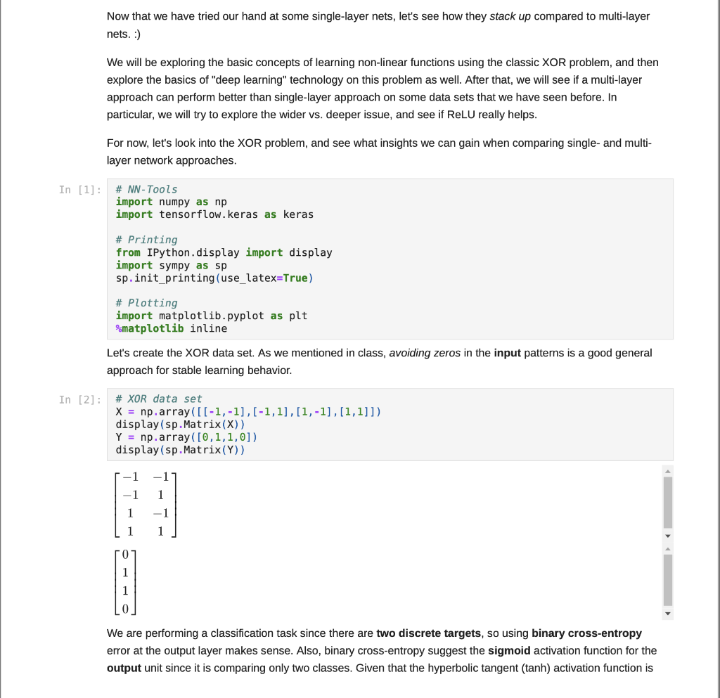
Step by Step Solution

There are 3 Steps involved in it

Step: 1

blur-text-image

Get Instant Access to Expert-Tailored Solutions

See step-by-step solutions with expert insights and AI powered tools for academic success

Step: 2

blur-text-image

Step: 3

blur-text-image

Ace Your Homework with AI

Get the answers you need in no time with our AI-driven, step-by-step assistance

Get Started

Recommended Textbook for

Big Data In Just 7 Chapters

Authors: Prof Marcus Vinicius Pinto

1st Edition

B09NZ7ZX72, 979-8787954036

More Books

Students also viewed these Databases questions

Question

b. Explain how you initially felt about the communication.

Answered: 1 week ago

Question

3. Identify the methods used within each of the three approaches.

Answered: 1 week ago

Question

a. When did your ancestors come to the United States?

Answered: 1 week ago