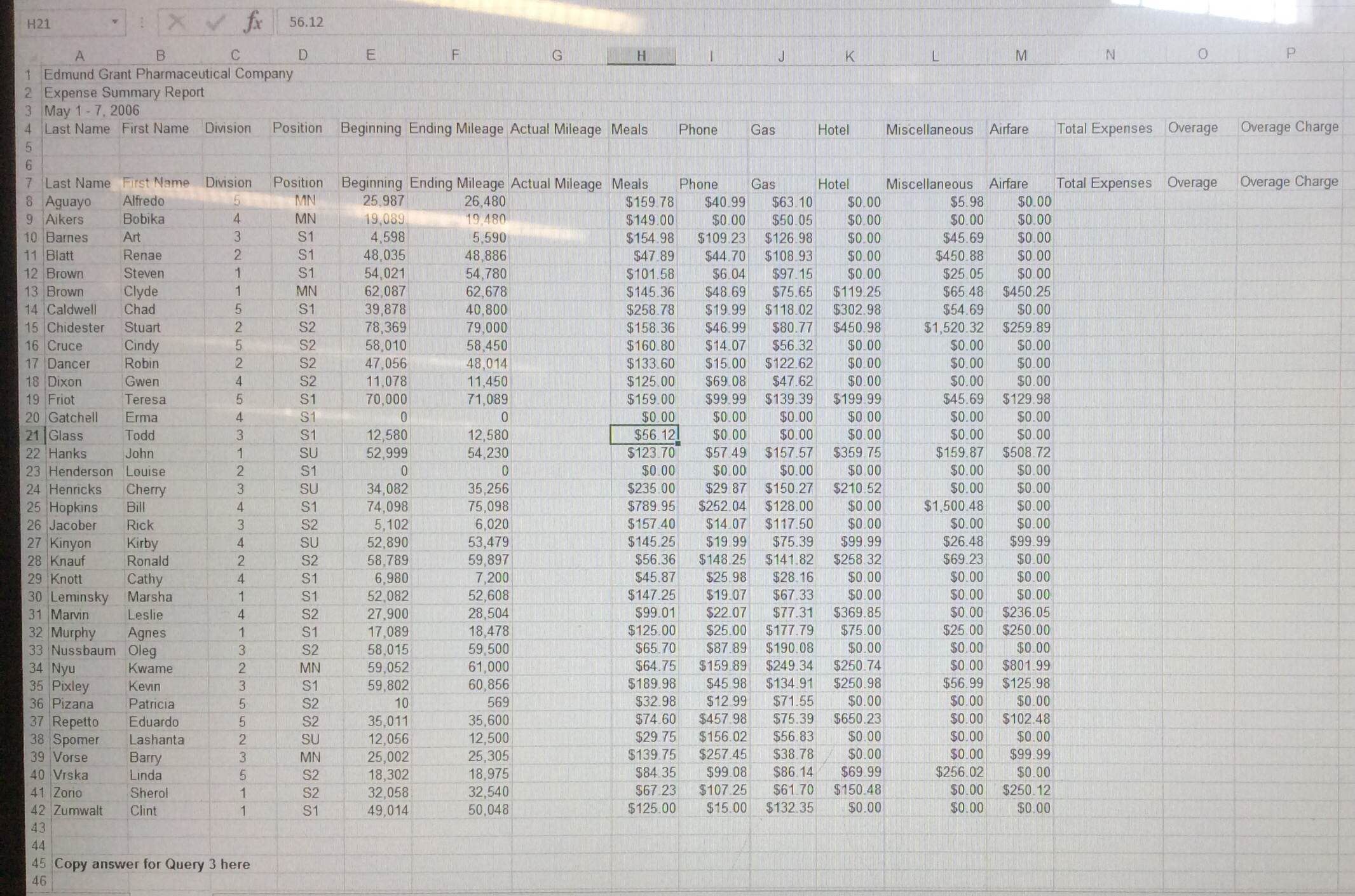
Keiko Lapeer is a district sales manager for the Edmund Grant Pharmaceutical Company. Each week, members of Ms. Lapeer's sales staff submit weekly expense claim forms. Currently, she scans through the expense forms, checks for anything out of the ordinary and then authorizes reimbursement checks. As this process is cumbersome and inefficient, you will be designing and analyzing an expenses worksheet that will allow Ms. Lapeer to easily track her sales staffs expenses.

Design Specifications

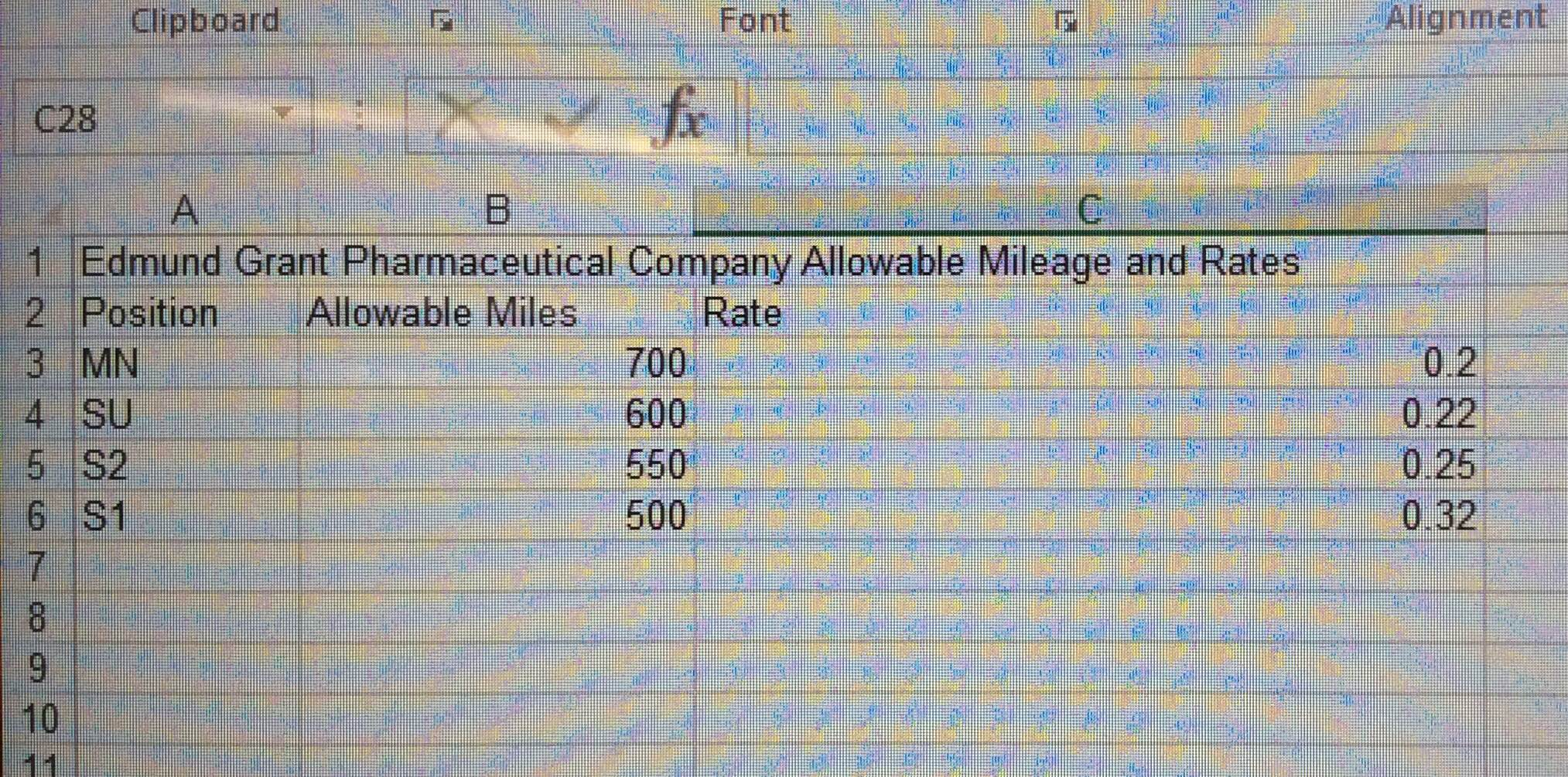
1. Carefully examine the data file. Notice that it contains two worksheets, one for expenses and another for mileage lookup information. Start by formatting the data table in the expenses worksheet (cells A7 through P42). Next, calculate the actual mileage, allowable miles, overage mileage, overage mileage rate, overage charge, and total expenses in the columns already provided in the worksheet. (Remember, the fill handle is your friend!) Refer to the following information:

Actual Mileage: The actual mileage column calculates the actual miles that each sales representative drove during the week. Actual mileage is the difference between the week's ending mileage and the week's beginning mileage.

Allowable Miles: Here, you will be matching up each sales representative with their corresponding allowable miles, which is based on their position. You will be using the VLOOKUP function to reference the mileage lookup table (in the lookup spreadsheet) to match up the sales representatives position with their corresponding allowable miles. Remember to lock the table_array input to prevent the selected table from shifting. (You can do this by pressing F4 when selecting the table_array input in the VLOOKUP function.)

VLOOKUP(lookup_value,table_array,col_index_number,range_lookup)

Overage Mileage: In order to find a sales representatives overage mileage, subtract their allowable miles from their actual mileage (i.e. Overage Mileage = Actual Mileage Allowable Miles). However, before trying to calculate overage mileage, you must realize that not every employee has exceeded their allowable miles. Note that simply using the above overage mileage formula for every sales representative will cause some sales representatives to have negative values for their overage mileage, meaning that they did not go over on their miles and actually had miles to spare. To show that these sales representatives did not go over their allowable miles (meaning, their overage mileage should be 0), you must use the IF function. The function will state: if the overage mileage that was just calculated is negative (i.e., less than 0) (logical_test), then display a 0 (value_if_true); otherwise, display the calculated overage mileage (value_if_false).

IF(logical_test, value_if_true, value_if_false)

Overage Mileage Rate: The overage mileage rate column uses the VLOOKUP function as well. Use the VLOOKUP function to find a sales representatives overage mileage rate from the mileage lookup table (in the lookup spreadsheet) based on their corresponding position.

Overage Charge: To find a sales representatives overage charge, multiply their overage mileage rate by their overage mileage.

Total Expenses: The total expenses column is simply the sum of a sales representatives meals, phone, gas, hotel, miscellaneous, and airfare expenses.

2. Ms. Lapeer wants to view the expense data at different levels of detail and from different perspectives. She specifically requests a summary of all total expenses for each sales division and total expenses for each sales position within each sales division. You will use the PivotTable tool to display the information accordingly.

First, select the entire expenses data table (cells A7 through P42). Then, under the Insert tab, click PivotTable. Make sure you are creating the PivotTable in a New Worksheet. Click OK.

You should now see a new worksheet containing a blank PivotTable and a PivotTable Field List (in a pane to the right of the worksheet) containing all the columns in the expenses data table. Drag the Division and Position fields (in that order) to the Row Labels box. This will display each position within each division. Next, drag the Total Expenses field to the Values box. This should now display the total expenses for each position within each division, the total expenses for each division, and the grand total of expenses for all the divisions.

P.S: if you can solve this issues problem by excel or any program. Would you mind to explain to me step by step and what formula did you use to solve it? I don't want only the answer but also learn how to do it.