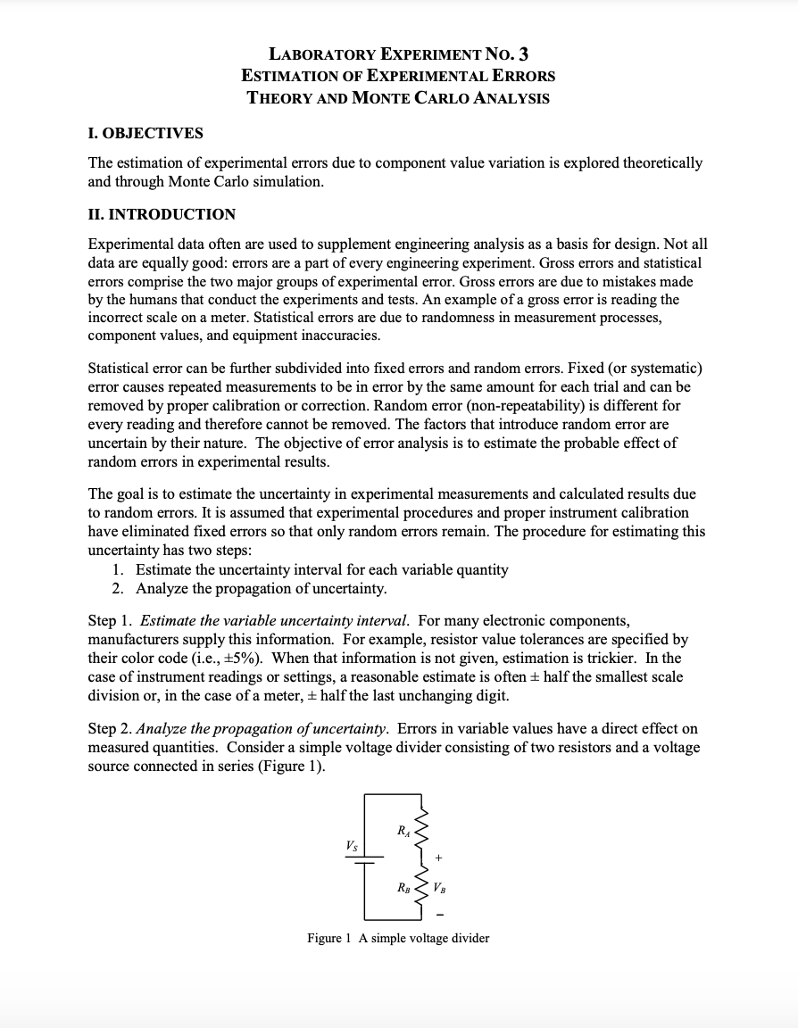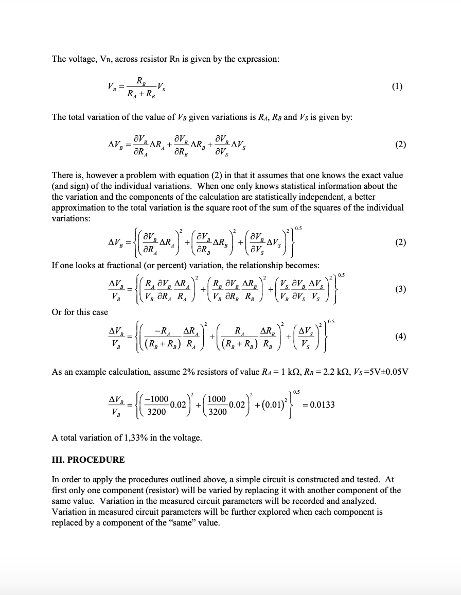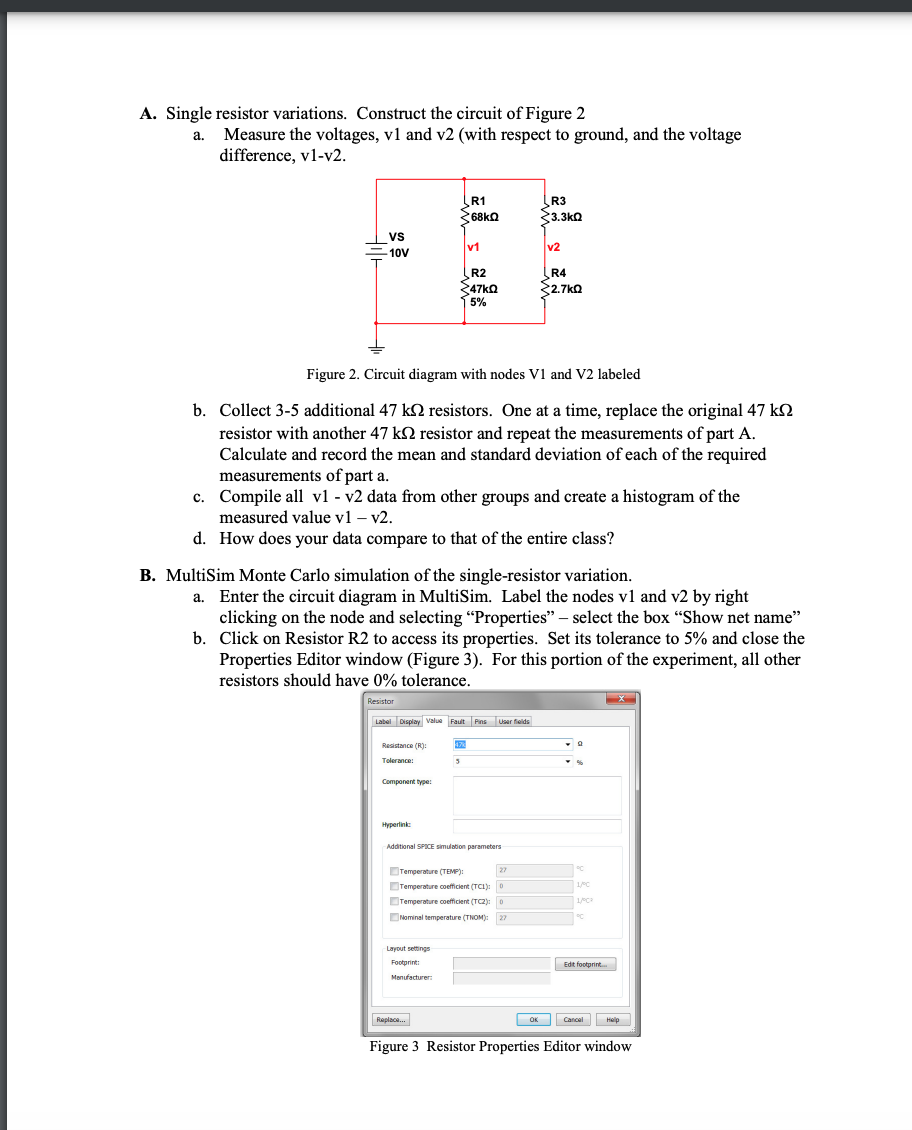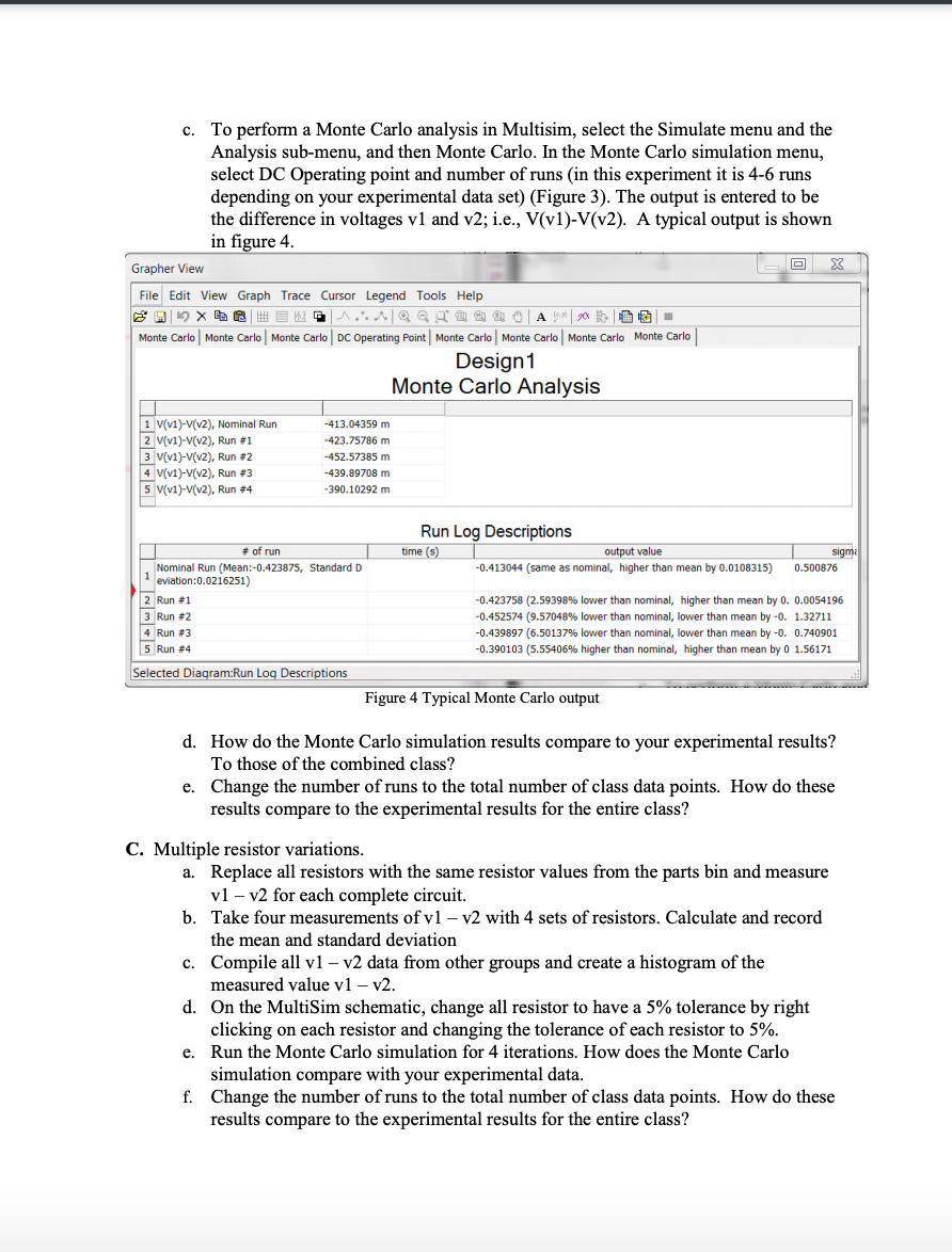
LABORATORY EXPERIMENT NO. 3 ESTIMATION OF EXPERIMENTAL ERRORS THEORY AND MONTE CARLO ANALYSIS I. OBJECTIVES The estimation of experimental errors due to component value variation is explored theoretically and through Monte Carlo simulation. II. INTRODUCTION Experimental data often are used to supplement engineering analysis as a basis for design. Not all data are equally good: errors are a part of every engineering experiment. Gross errors and statistical errors comprise the two major groups of experimental error. Gross errors are due to mistakes made by the humans that conduct the experiments and tests. An example of a gross error is reading the incorrect scale on a meter. Statistical errors are due to randomness in measurement processes, component values, and equipment inaccuracies. Statistical error can be further subdivided into fixed errors and random errors. Fixed (or systematic) error causes repeated measurements to be in error by the same amount for each trial and can be removed by proper calibration or correction. Random error (non-repeatability) is different for every reading and therefore cannot be removed. The factors that introduce random error are uncertain by their nature. The objective of error analysis is to estimate the probable effect of random errors in experimental results. The goal is to estimate the uncertainty in experimental measurements and calculated results due to random errors. It is assumed that experimental procedures and proper instrument calibration have eliminated fixed errors so that only random errors remain. The procedure for estimating this uncertainty has two steps: 1. Estimate the uncertainty interval for each variable quantity 2. Analyze the propagation of uncertainty. Step 1. Estimate the variable uncertainty interval. For many electronic components, manufacturers supply this information. For example, resistor value tolerances are specified by their color code (i.e., +5%). When that information is not given, estimation is trickier. In the case of instrument readings or settings, a reasonable estimate is often + half the smallest scale division or, in the case of a meter, half the last unchanging digit. Step 2. Analyze the propagation of uncertainty. Errors in variable values have a direct effect on measured quantities. Consider a simple voltage divider consisting of two resistors and a voltage source connected in series (Figure 1). R VS RR Figure 1 A simple voltage divider The voltage, VB, across resistor RB is given by the expression: RE V,= BV RA+R (1) The total variation of the value of VB given variations is RA, RB and Vs is given by: , av av av -AR + AR + OR OR; avs B AVS (2) There is, however a problem with equation (2) in that it assumes that one knows the exact value (and sign) of the individual variations. When one only knows statistical information about the the variation and the components of the calculation are statistically independent, a better approximation to the total variation is the square root of the sum of the squares of the individual variations: 0.5 OVB ARA + OVB ARB OR: .)-( }} (2) ORA av AVE = -AVS av If one looks at fractional (or percent) variation, the relationship becomes: AV R, OV, AR R, OV, AR V, OV, AV V, ORRA V, OR, RB V, av, vs Or for this case 0.5 + (3) 05 AV , -R AR (R+R3) R + RA AR (Rg+Rx) Ry , V (4) As an example calculation, assume 2% resistors of value RA= 1 k-2, RB = 2.2 k2, Vs=5V+0.05V 0.5 AV VE -1000 -0.02 3200 1000 -0.02 +0.01) 3200 = 0.0133 A total variation of 1,33% in the voltage. III. PROCEDURE In order to apply the procedures outlined above, a simple circuit is constructed and tested. At first only one component (resistor) will be varied by replacing it with another component of the same value. Variation in the measured circuit parameters will be recorded and analyzed. Variation in measured circuit parameters will be further explored when each component is replaced by a component of the same" value. A. Single resistor variations. Construct the circuit of Figure 2 Measure the voltages, vl and v2 (with respect to ground, and the voltage difference, vl-v2. a. R3 R1 68k 33.3k Holt VS 10V v1 v2 R2 47k 5% R4 2.7k Figure 2. Circuit diagram with nodes V1 and V2 labeled b. Collect 3-5 additional 47 k 2 resistors. One at a time, replace the original 47 k12 resistor with another 47 k2 resistor and repeat the measurements of part A. Calculate and record the mean and standard deviation of each of the required measurements of part a. c. Compile all vl - v2 data from other groups and create a histogram of the measured value v1 - v2. d. How does your data compare to that of the entire class? a. B. MultiSim Monte Carlo simulation of the single-resistor variation. Enter the circuit diagram in MultiSim. Label the nodes vl and v2 by right clicking on the node and selecting Properties select the box "Show net name" b. Click on Resistor R2 to access its properties. Set its tolerance to 5% and close the Properties Editor window (Figure 3). For this portion of the experiment, all other resistors should have 0% tolerance. Resistor Label Display Value Fault Pins User fields 178 Resistance(): Tolerance 5 3 Component type: Hyperlink Additional SPICE simulation parameters 1 Temperature (TEM) 22 Temperature coefficient (TCI): 0 Temperature coefficient (TC): 0 Nominal temperature (TNOM): 27 1 Layout settings Footprint: Manufacturer: Edt footprint Replace... OK Cancel Help Figure 3 Resistor Properties Editor window c. To perform a Monte Carlo analysis in Multisim, select the Simulate menu and the Analysis sub-menu, and then Monte Carlo. In the Monte Carlo simulation menu, select DC Operating point and number of runs in this experiment it is 4-6 runs depending on your experimental data set) (Figure 3). The output is entered to be the difference in voltages vl and v2; i.e., V(v1)-V(v2). A typical output is shown in figure 4. X Grapher View File Edit View Graph Trace Cursor Legend Tools Help 3 x 2 L HH = Gege @ @ OA 09 Monte Carlo Monte Carlo Monte Carlo DC Operating Point Monte Carlo Monte Carlo Monte Carlo Monte Carlo Design1 Monte Carlo Analysis 1 V(v1)-V(v2), Nominal Run 2 V(v1)-V(v2), Run #1 3 V(v1)-V(v2), Run #2 4 V(v1)-V(v2), Run #3 5 V(v1)-V(v2), Run #4 -413.04359 m -423.75786 m -452.57385 m -439.89708 m -390.10292 m Run Log Descriptions # of run time (s) output value sigmi Nominal Run (Mean:-0.423875, Standard D -0.413044 (same as nominal, higher than mean by 0.0108315) 0.500876 eviation:0.0216251) Run #1 -0.423758 (2.59398% lower than nominal, higher than mean by 0. 0.0054196 3 Run #2 -0.452574 (9.57048% lower than nominal, lower than mean by -0. 1.32711 4 Run #3 -0.439897 (6.50137% lower than nominal, lower than mean by -0. 0.740901 5 Run 24 -0.390103 (5.55406% higher than nominal, higher than mean by 0 1.56171 Selected Diagram:Run Log Descriptions Figure 4 Typical Monte Carlo output d. How do the Monte Carlo simulation results compare to your experimental results? To those of the combined class? e. Change the number of runs to the total number of class data points. How do these results compare to the experimental results for the entire class? C. Multiple resistor variations. a. Replace all resistors with the same resistor values from the parts bin and measure vl - v2 for each complete circuit. b. Take four measurements of v1 - v2 with 4 sets of resistors. Calculate and record the mean and standard deviation c. Compile all vl - v2 data from other groups and create a histogram of the measured value vl-v2. d. On the MultiSim schematic, change all resistor to have a 5% tolerance by right clicking on each resistor and changing the tolerance of each resistor to 5%. e. Run the Monte Carlo simulation for 4 iterations. How does the Monte Carlo simulation compare with your experimental data. f. Change the number of runs to the total number of class data points. How do these results compare to the experimental results for the entire class? LABORATORY EXPERIMENT NO. 3 ESTIMATION OF EXPERIMENTAL ERRORS THEORY AND MONTE CARLO ANALYSIS I. OBJECTIVES The estimation of experimental errors due to component value variation is explored theoretically and through Monte Carlo simulation. II. INTRODUCTION Experimental data often are used to supplement engineering analysis as a basis for design. Not all data are equally good: errors are a part of every engineering experiment. Gross errors and statistical errors comprise the two major groups of experimental error. Gross errors are due to mistakes made by the humans that conduct the experiments and tests. An example of a gross error is reading the incorrect scale on a meter. Statistical errors are due to randomness in measurement processes, component values, and equipment inaccuracies. Statistical error can be further subdivided into fixed errors and random errors. Fixed (or systematic) error causes repeated measurements to be in error by the same amount for each trial and can be removed by proper calibration or correction. Random error (non-repeatability) is different for every reading and therefore cannot be removed. The factors that introduce random error are uncertain by their nature. The objective of error analysis is to estimate the probable effect of random errors in experimental results. The goal is to estimate the uncertainty in experimental measurements and calculated results due to random errors. It is assumed that experimental procedures and proper instrument calibration have eliminated fixed errors so that only random errors remain. The procedure for estimating this uncertainty has two steps: 1. Estimate the uncertainty interval for each variable quantity 2. Analyze the propagation of uncertainty. Step 1. Estimate the variable uncertainty interval. For many electronic components, manufacturers supply this information. For example, resistor value tolerances are specified by their color code (i.e., +5%). When that information is not given, estimation is trickier. In the case of instrument readings or settings, a reasonable estimate is often + half the smallest scale division or, in the case of a meter, half the last unchanging digit. Step 2. Analyze the propagation of uncertainty. Errors in variable values have a direct effect on measured quantities. Consider a simple voltage divider consisting of two resistors and a voltage source connected in series (Figure 1). R VS RR Figure 1 A simple voltage divider The voltage, VB, across resistor RB is given by the expression: RE V,= BV RA+R (1) The total variation of the value of VB given variations is RA, RB and Vs is given by: , av av av -AR + AR + OR OR; avs B AVS (2) There is, however a problem with equation (2) in that it assumes that one knows the exact value (and sign) of the individual variations. When one only knows statistical information about the the variation and the components of the calculation are statistically independent, a better approximation to the total variation is the square root of the sum of the squares of the individual variations: 0.5 OVB ARA + OVB ARB OR: .)-( }} (2) ORA av AVE = -AVS av If one looks at fractional (or percent) variation, the relationship becomes: AV R, OV, AR R, OV, AR V, OV, AV V, ORRA V, OR, RB V, av, vs Or for this case 0.5 + (3) 05 AV , -R AR (R+R3) R + RA AR (Rg+Rx) Ry , V (4) As an example calculation, assume 2% resistors of value RA= 1 k-2, RB = 2.2 k2, Vs=5V+0.05V 0.5 AV VE -1000 -0.02 3200 1000 -0.02 +0.01) 3200 = 0.0133 A total variation of 1,33% in the voltage. III. PROCEDURE In order to apply the procedures outlined above, a simple circuit is constructed and tested. At first only one component (resistor) will be varied by replacing it with another component of the same value. Variation in the measured circuit parameters will be recorded and analyzed. Variation in measured circuit parameters will be further explored when each component is replaced by a component of the same" value. A. Single resistor variations. Construct the circuit of Figure 2 Measure the voltages, vl and v2 (with respect to ground, and the voltage difference, vl-v2. a. R3 R1 68k 33.3k Holt VS 10V v1 v2 R2 47k 5% R4 2.7k Figure 2. Circuit diagram with nodes V1 and V2 labeled b. Collect 3-5 additional 47 k 2 resistors. One at a time, replace the original 47 k12 resistor with another 47 k2 resistor and repeat the measurements of part A. Calculate and record the mean and standard deviation of each of the required measurements of part a. c. Compile all vl - v2 data from other groups and create a histogram of the measured value v1 - v2. d. How does your data compare to that of the entire class? a. B. MultiSim Monte Carlo simulation of the single-resistor variation. Enter the circuit diagram in MultiSim. Label the nodes vl and v2 by right clicking on the node and selecting Properties select the box "Show net name" b. Click on Resistor R2 to access its properties. Set its tolerance to 5% and close the Properties Editor window (Figure 3). For this portion of the experiment, all other resistors should have 0% tolerance. Resistor Label Display Value Fault Pins User fields 178 Resistance(): Tolerance 5 3 Component type: Hyperlink Additional SPICE simulation parameters 1 Temperature (TEM) 22 Temperature coefficient (TCI): 0 Temperature coefficient (TC): 0 Nominal temperature (TNOM): 27 1 Layout settings Footprint: Manufacturer: Edt footprint Replace... OK Cancel Help Figure 3 Resistor Properties Editor window c. To perform a Monte Carlo analysis in Multisim, select the Simulate menu and the Analysis sub-menu, and then Monte Carlo. In the Monte Carlo simulation menu, select DC Operating point and number of runs in this experiment it is 4-6 runs depending on your experimental data set) (Figure 3). The output is entered to be the difference in voltages vl and v2; i.e., V(v1)-V(v2). A typical output is shown in figure 4. X Grapher View File Edit View Graph Trace Cursor Legend Tools Help 3 x 2 L HH = Gege @ @ OA 09 Monte Carlo Monte Carlo Monte Carlo DC Operating Point Monte Carlo Monte Carlo Monte Carlo Monte Carlo Design1 Monte Carlo Analysis 1 V(v1)-V(v2), Nominal Run 2 V(v1)-V(v2), Run #1 3 V(v1)-V(v2), Run #2 4 V(v1)-V(v2), Run #3 5 V(v1)-V(v2), Run #4 -413.04359 m -423.75786 m -452.57385 m -439.89708 m -390.10292 m Run Log Descriptions # of run time (s) output value sigmi Nominal Run (Mean:-0.423875, Standard D -0.413044 (same as nominal, higher than mean by 0.0108315) 0.500876 eviation:0.0216251) Run #1 -0.423758 (2.59398% lower than nominal, higher than mean by 0. 0.0054196 3 Run #2 -0.452574 (9.57048% lower than nominal, lower than mean by -0. 1.32711 4 Run #3 -0.439897 (6.50137% lower than nominal, lower than mean by -0. 0.740901 5 Run 24 -0.390103 (5.55406% higher than nominal, higher than mean by 0 1.56171 Selected Diagram:Run Log Descriptions Figure 4 Typical Monte Carlo output d. How do the Monte Carlo simulation results compare to your experimental results? To those of the combined class? e. Change the number of runs to the total number of class data points. How do these results compare to the experimental results for the entire class? C. Multiple resistor variations. a. Replace all resistors with the same resistor values from the parts bin and measure vl - v2 for each complete circuit. b. Take four measurements of v1 - v2 with 4 sets of resistors. Calculate and record the mean and standard deviation c. Compile all vl - v2 data from other groups and create a histogram of the measured value vl-v2. d. On the MultiSim schematic, change all resistor to have a 5% tolerance by right clicking on each resistor and changing the tolerance of each resistor to 5%. e. Run the Monte Carlo simulation for 4 iterations. How does the Monte Carlo simulation compare with your experimental data. f. Change the number of runs to the total number of class data points. How do these results compare to the experimental results for the entire class