Lagrange-2.m :

function y=Lagrange(xi,fi,x)

% data: (xi,fi), i=0, ...,n

% evaluation points: x

% return: y=p(x), where p is the interpolant

n=length(xi)-1;

y=zeros(size(x));

for k=0:n

num=ones(size(x));

den=1;

for j=0:k-1

num=num.*(x-xi(j+1));

den=den*(xi(k+1)-xi(j+1));

end

for j=k+1:n

num=num.*(x-xi(j+1));

den=den*(xi(k+1)-xi(j+1));

end

l=num/den;

y=y+fi(k+1).*l;

end

Just need the Matlab Code, Thanks.

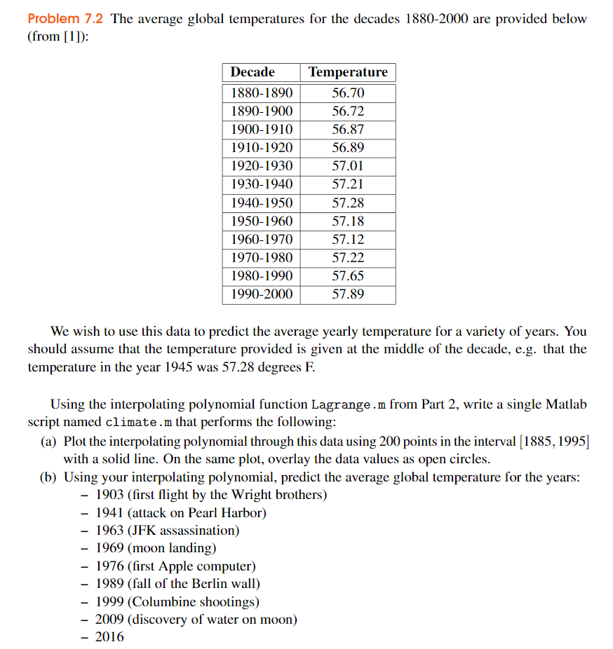
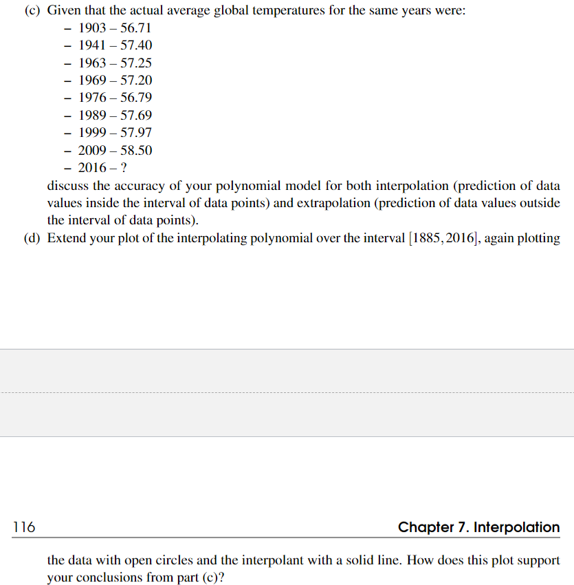
Problem 7.2 The average global temperatures for the decades 1880-2000 are provided below (from [1]: Decade 1880-1890 1890-1900 1900-1910 1910-1920 1920-1930 1930-1940 1940-1950 1950-1960 1960-1970 1970-1980 1980-1990 1990-2000 Temperature 56.70 56.72 56.87 56.89 57.01 57.21 57.28 57.18 57.12 57.22 57.65 57.89 We wish to use this data to predict the average yearly temperature for a variety of years. You should assume that the temperature provided is given at the middle of the decade, e.g. that the temperature in the year 1945 was 57.28 degrees F. Using the interpolating polynomial function Lagrange.m from Part 2, write a single Matlab script named climate.m that performs the following: (a) Plot the interpolating polynomial through this data using 200 points in the interval (1885, 1995] with a solid line. On the same plot, overlay the data values as open circles. (b) Using your interpolating polynomial, predict the average global temperature for the years: 1903 (first flight by the Wright brothers) - 1941 (attack on Pearl Harbor) 1963 (JFK assassination) - 1969 (moon landing) 1976 (first Apple computer) - 1989 (fall of the Berlin wall) - 1999 (Columbine shootings) 2009 (discovery of water on moon) - 2016 (c) Given that the actual average global temperatures for the same years were: - 1903 56.71 - 1941 - 57.40 - 1963 57.25 - 1969 - 57.20 - 1976 - 56.79 - 1989 - 57.69 - 1999 - 57.97 - 2009 - 58.50 - 2016 - ? discuss the accuracy of your polynomial model for both interpolation (prediction of data values inside the interval of data points) and extrapolation (prediction of data values outside the interval of data points). (d) Extend your plot of the interpolating polynomial over the interval (1885, 2016), again plotting 116 Chapter 7. Interpolation the data with open circles and the interpolant with a solid line. How does this plot support your conclusions from part (c)