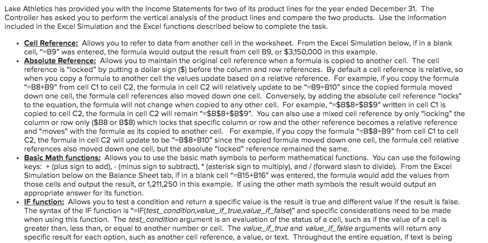
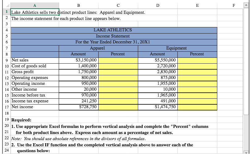
Lake Athletics has provided you with the Income Statements for two of its product lines for the year ended December 31. The Controller has asked you to perform the vertical analysis of the product lines and compare the two products. Use the information included in the Excel Simulation and the Excel functions described below to complete the task. Cell Reference: Allows you to refer to data from another cell in the worksheet. From the Excel Simulation below, if in a blank cell, "=B9" was entered, the formula would output the result from cell B9, or $3,150,000 in this example. Absolute Reference: Allows you to maintain the original cell reference when a formula is copied to another cell. The cell reference is "locked" by putting a dollar sign ($) before the column and row references. By default a cell reference is relative, so when you copy a formula to another cell the values update based on a relative reference. For example, if you copy the formula "=B8+B9" from cell C1 to cell C2, the formula in cell C2 will relatively update to be "=B9+B10" since the copied formula moved down one cell, the formula cell references also moved down one cell. Conversely, by adding the absolute cell reference "locks" to the equation, the formula will not change when copied to any other cell. For example, "=$B$8+$B$9" written in cell C1 is copied to cell C2, the formula in cell C2 will remain "=$B$8+$B$9". You can also use a mixed cell reference by only "locking" the column or row only ($B8 or B$8) which locks that specific column or row and the other reference becomes a relative reference and "moves" with the formula as its copied to another cell. For example, if you copy the formula "=B$8+B9" from cell C1 to cell C2, the formula in cell C2 will update to be "=B$8+B10" since the copied formula moved down one cell, the formula cell relative references also moved down one cell, but the absolute "locked" reference remained the same. Basic Math functions: Allows you to use the basic math symbols to perform mathematical functions. You can use the following keys: + (plus sign to add), - (minus sign to subtract), * (asterisk sign to multiply), and / (forward slash to divide). From the Excel Simulation below on the Balance Sheet tab, if in a blank cell "=B15+B16" was entered, the formula would add the values from those cells and output the result, or 1,211,250 in this example. If using the other math symbols the result would output an appropriate answer for its function. IF function: Allows you to test a condition and return a specific value is the result is true and different value if the result is false. The syntax of the IF function is "=IF(test_condition,value_if_true,value_if_false)" and specific considerations need to be made when using this function. The test condition argument is an evaluation of the status of a cell, such as if the value of a cell is greater than, less than, or equal to another number or cell. The value_if_true and value_if_false arguments will return any specific result for each option, such as another cell reference, a value, or text. Throughout the entire equation, if text is being 1 Lake Athletics sells two distinct product lines: Apparel and Equipment. 2 The income statement for each product line appears below. Percent 9 Net sales 10 Cost of goods sold 11 Gross profit 12 Operating expenses 13 Operating income 14 Other income 15 Income before tax 16 Income tax expense 17 Net income LAKE ATHLETICS Income Statement For the Year Ended December 31, 20X1 Apparel Equipment Amount Percent Amount $3,150,000 $5,550,000 1,400,000 2,720,000 1,750,000 2,830,000 800,000 875,000 950,000 1,955,000 20,000 10,000 970,000 1,965,000 241,250 491,000 $728,750 $1,474,750 D C 19 Required: 20 1. Use appropriate Excel formulas to perform vertical analysis and complete the "Percent" columns for both product lines above. Express each amount as a percentage of net sales. 22 Note: You should use absolute references in the divisors of all formulas. 23 2. Use the Excel IF function and the completed vertical analysis above to answer each of the 24 questions below: Which product line has the highest gross profit %? Which product line has the highest net income %