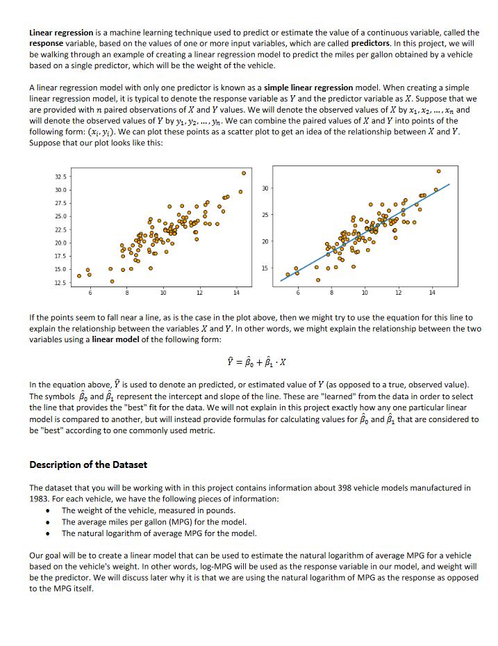
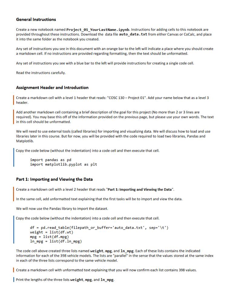
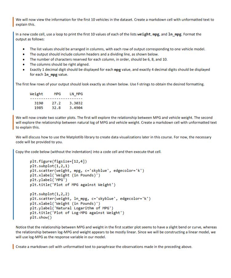
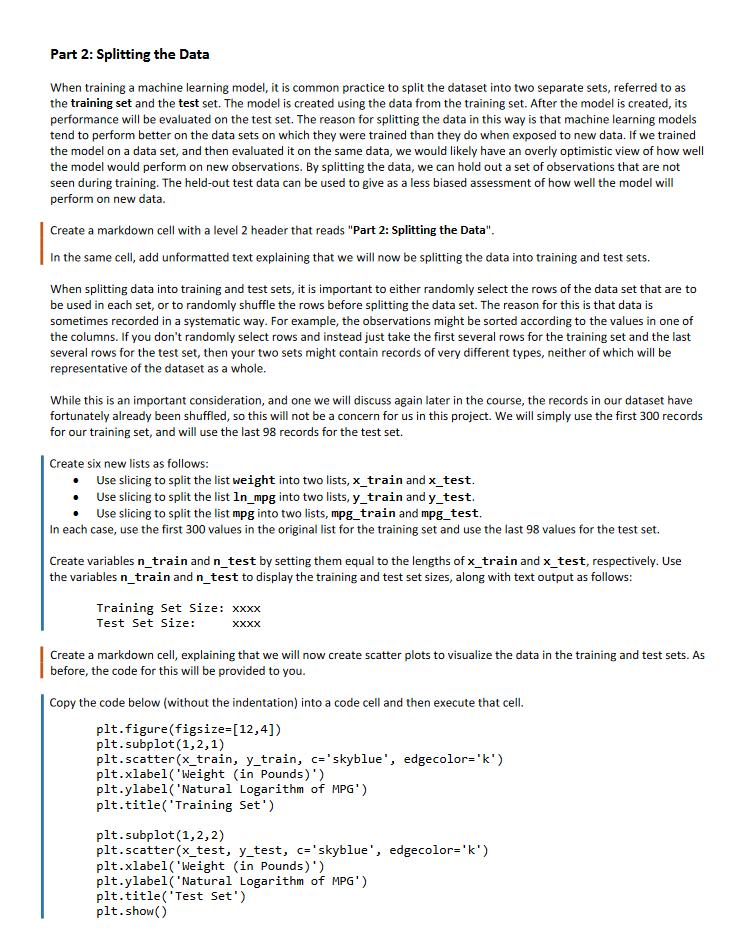
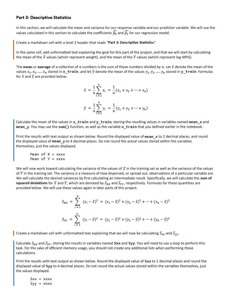
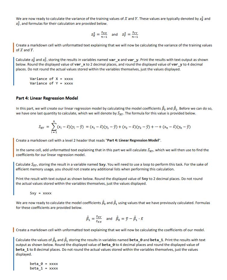
Linear regression is a machine learning technique used to predict or estimate the value of a continuous variable, called the response variable, based on the values of one or more input variables, which are called predictors. In this project, we will be walking through an example of creating a linear regression model to predict the miles per gallon obtained by a vehicle based on a single predictor, which will be the weight of the vehicle. A linear regression model with only one predictor is known as a simple linear regression model. When creating a simple linear regression model, it is typical to denote the response variable as Y and the predictor variable as X. Suppose that we are provided with n paired observations of X and Y values. We will denote the observed values of X by x1, x2,..., X and will denote the observed values of Y by y1 y2.... h. We can combine the paired values of X and Y into points of the following form: (x, y). We can plot these points as a scatter plot to get an idea of the relationship between X and Y. Suppose that our plot looks like this: 32.5 30.0 27.5 25.0 22.5 20.0 17.5 15.0 12.5 14 30 10 20 15 12 14 If the points seem to fall near a line, as is the case in the plot above, then we might try to use the equation for this line to explain the relationship between the variables X and Y. In other words, we might explain the relationship between the two variables using a linear model of the following form: In the equation above, is used to denote an predicted, or estimated value of Y (as opposed to a true, observed value). The symbols B and B represent the intercept and slope of the line. These are "learned" from the data in order to select the line that provides the "best" fit for the data. We will not explain in this project exactly how any one particular linear model is compared to another, but will instead provide formulas for calculating values for o and B that are considered to be "best" according to one commonly used metric. Description of the Dataset The dataset that you will be working with in this project contains information about 398 vehicle models manufactured in 1983. For each vehicle, we have the following pieces of information: The weight of the vehicle, measured in pounds. The average miles per gallon (MPG) for the model. The natural logarithm of average MPG for the model. Our goal will be to create a linear model that can be used to estimate the natural logarithm of average MPG for a vehicle based on the vehicle's weight. In other words, log-MPG will be used as the response variable in our model, and weight will be the predictor. We will discuss later why it is that we are using the natural logarithm of MPG as the response as opposed to the MPG itself. General Instructions Create a new notebook named Project_01_YourLastName.ipynb. Instructions for adding cells to this notebook are provided throughout these instructions. Download the data file auto_data.txt from either Canvas or CoCalc, and place it into the same folder as the notebook you created. Any set of instructions you see in this document with an orange bar to the left will indicate a place where you should create a markdown cell. If no instructions are provided regarding formatting, then the text should be unformatted. Any set of instructions you see with a blue bar to the left will provide instructions for creating a single code cell. Read the instructions carefully. Assignment Header and Introduction Create a markdown cell with a level 1 header that reads: "COSC 130-Project 01". Add your name below that as a level 3 header. Add another markdown cell containing a brief description of the goal for this project (No more than 2 or 3 lines are required). You may base this off of the information provided on the previous page, but please use your own words. The text in this cell should be unformatted. We will need to use external tools (called libraries) for importing and visualizing data. We will discuss how to load and use libraries later in this course. But for now, you will be provided with the code required to load two libraries, Pandas and Matplotlib. Copy the code below (without the indentation) into a code cell and then execute that cell. import pandas as pd import matplotlib.pyplot as plt Part 1: Importing and Viewing the Data Create a markdown cell with a level 2 header that reads "Part 1: Importing and Viewing the Data". In the same cell, add unformatted text explaining that the first tasks will be to import and view the data. We will now use the Pandas library to import the dataset. Copy the code below (without the indentation) into a code cell and then execute that cell. df pd.read_table(filepath_or_buffer="auto_data.txt', sep='\t') weight = list(df.wt) mpg list(df.mpg) In mpg list(df. 1n_mpg) The code cell above created three lists named weight, mpg, and 1n_mpg. Each of these lists contains the indicated information for each of the 398 vehicle models. The lists are "parallel" in the sense that the values stored at the same index in each of the three lists correspond to the same vehicle model. Create a markdown cell with unformatted text explaining that you will now confirm each list contains 398 values. Print the lengths of the three lists weight, mpg, and 1n_mpg. We will now view the information for the first 10 vehicles in the dataset. Create a markdown cell with unformatted text to explain this. In a new code cell, use a loop to print the first 10 values of each of the lists weight, mpg, and In_mpg. Format the output as follows: The list values should be arranged in columns, with each row of output corresponding to one vehicle model. The output should include column headers and a dividing line, as shown below. The number of characters reserved for each column, in order, should be 6, 8, and 10. The columns should be right aligned. Exactly 1 decimal digit should be displayed for each mpg value, and exactly 4 decimal digits should be displayed for each In mpg value. The first few rows of your output should look exactly as shown below. Use f-strings to obtain the desired formatting. Weight MPG LN_MPG 3190 1985 27.2 32.8 3.3032 3.4904 We will now create two scatter plots. The first will explore the relationship between MPG and vehicle weight. The second will explore the relationship between natural log of MPG and vehicle weight. Create a markdown cell with unformatted text to explain this. We will discuss how to use the Matplotlib library to create data visualizations later in this course. For now, the necessary code will be provided to you. Copy the code below (without the indentation) into a code cell and then execute that cell. plt.figure(figsize=[12,4]) plt.subplot(1,2,1) plt.scatter (weight, mpg, c='skyblue', edgecolor='k') plt.xlabel('Weight (in Pounds)') plt.ylabel('MPG') plt.title('Plot of MPG against Weight') plt.subplot(1,2,2) plt.scatter (weight, 1n_mpg, c='skyblue', edgecolor='k') plt.xlabel('Weight (in Pounds)') plt.ylabel('Natural Logarithm of MPG') plt.title('Plot of Log-MPG against Weight') plt.show() Notice that the relationship between MPG and weight in the first scatter plot seems to have a slight bend or curve, whereas the relationship between log-MPG and weight appears to be mostly linear. Since we will be constructing a linear model, we will use log-MPG as the response variable in our model. Create a markdown cell with unformatted text to paraphrase the observations made in the preceding above. Part 2: Splitting the Data When training a machine learning model, it is common practice to split the dataset into two separate sets, referred to as the training set and the test set. The model is created using the data from the training set. After the model is created, its performance will be evaluated on the test set. The reason for splitting the data in this way is that machine learning models tend to perform better on the data sets on which they were trained than they do when exposed to new data. If we trained the model on a data set, and then evaluated it on the same data, we would likely have an overly optimistic view of how well the model would perform on new observations. By splitting the data, we can hold out a set of observations that are not seen during training. The held-out test data can be used to give as a less biased assessment of how well the model will perform on new data. Create a markdown cell with a level 2 header that reads "Part 2: Splitting the Data". In the same cell, add unformatted text explaining that we will now be splitting the data into training and test sets. When splitting data into training and test sets, it is important to either randomly select the rows of the data set that are to be used in each set, or to randomly shuffle the rows before splitting the data set. The reason for this is that data is sometimes recorded in a systematic way. For example, the observations might be sorted according to the values in one of the columns. If you don't randomly select rows and instead just take the first several rows for the training set and the last several rows for the test set, then your two sets might contain records of very different types, neither of which will be representative of the dataset as a whole. While this is an important consideration, and one we will discuss again later in the course, the records in our dataset have fortunately already been shuffled, so this will not be a concern for us in this project. We will simply use the first 300 records for our training set, and will use the last 98 records for the test set. Create six new lists as follows: Use slicing to split the list weight into two lists, x_train and x_test. Use slicing to split the list In_mpg into two lists, y_train and y_test. Use slicing to split the list mpg into two lists, mpg_train and mpg_test. In each case, use the first 300 values in the original list for the training set and use the last 98 values for the test set. Create variables n_train and n_test by setting them equal to the lengths of x_train and x_test, respectively. Use the variables n_train and n_test to display the training and test set sizes, along with text output as follows: Training Set Size: xxxx Test Set Size: XXXX Create a markdown cell, explaining that we will now create scatter plots to visualize the data in the training and test sets. As before, the code for this will be provided to you. Copy the code below (without the indentation) into a code cell and then execute that cell. plt.figure(figsize=[12,4]) plt.subplot(1,2,1) plt.scatter (x_train, y_train, c='skyblue', edgecolor='k') plt.xlabel('Weight (in Pounds)') plt.ylabel('Natural Logarithm of MPG') plt.title('Training Set') plt.subplot(1,2,2) plt.scatter (x_test, y_test, c='skyblue', edgecolor='k') plt.xlabel('Weight (in Pounds)') plt.ylabel('Natural Logarithm of MPG') plt.title('Test Set') plt.show() Part 3: Descriptive Statistics In this section, we will calculate the mean and variance for our response variable and our predictor variable. We will use the values calculated in this section to calculate the coefficients Bo and B for our regression model. Create a markdown cell with a level 2 header that reads "Part 3: Descriptive Statistics". In the same cell, add unformatted text explaining the goal for this part of the project, and that we will start by calculating the mean of the X values (which represent weight), and the mean of the Y values (which represent log-MPG). The mean or average of a collection of n numbers is the sum of those numbers divided by n. Let x denote the mean of the values x1, x2, stored in x_train, and let y denote the mean of the values y.2....y stored in y_train. Formulas for x and y are provided below. x = n x = 1 y y = Calculate the mean of the values in x_train and y_train, storing the resulting values in variables named mean_x and mean_y. You may use the sum() function, as well as the variable n_train that you defined earlier in the notebook. Print the results with text output as shown below. Round the displayed value of mean_x to 2 decimal places, and round the displayed value of mean_y to 4 decimal places. Do not round the actual values stored within the variables themselves, just the values displayed. Mean of X Mean of Y XXXX xXXX We will now work toward calculating the variance of the values of X in the training set as well as the variance of the values of Y in the training set. The variance is a measure of how dispersed, or spread out, observations of a particular variable are. We will calculate the desired variances by first calculating an intermediate result. Specifically, we will calculate the sum of squared deviations for X and Y, which are denoted by Sxx and Syy, respectively. Formulas for these quantities are provided below. We will use these values again in later parts of this project. n Sxx = (xx) = (x x) + (x x) + ... + (x x) i=1 71 - Syy = (1) = (1 1) + (2 1) + + (n 1) i=1 Create a markdown cell with unformatted text explaining that we will now be calculating 5xx and Syy. Calculate Sxx and Syy, storing the results in variables named Sxx and Syy. You will need to use a loop to perform this task. For the sake of efficient memory usage, you should not create any additional lists when performing these calculations. Print the results with text output as shown below. Round the displayed value of Sxx to 2 decimal places and round the displayed value of Syy to 4 decimal places. Do not round the actual values stored within the variables themselves, just the values displayed. Sxx = XXXX Syy = xxxx We are now ready to calculate the variance of the training values of X and Y. These values are typically denoted by sand s, and formulas for their calculation are provided below. = Sxx n-1 Syy and s = n-1 Create a markdown cell with unformatted text explaining that we will now be calculating the variance of the training values of X and Y. Calculate sand s, storing the results in variables named var_x and vary. Print the results with text output as shown below. Round the displayed value of var_x to 2 decimal places, and round the displayed value of var_y to 4 decimal places. Do not round the actual values stored within the variables themselves, just the values displayed. Variance of X = xxxx Variance of Y = xxxx Part 4: Linear Regression Model In this part, we will create our linear regression model by calculating the model coefficients o and B. Before we can do so, we have one last quantity to calculate, which we will denote by Sxy. The formula for this value is provided below. Sxy = (x ) ( 1) = (x x) (V ) + (x2 x) (V2 ) + + (x x)(Yn 1) i=1 Create a markdown cell with a level 2 header that reads "Part 4: Linear Regression Model. In the same cell, add unformatted text explaining that in this part we will calculate Sxy, which we will then use to find the coefficients for our linear regression model. Calculate Sxy, storing the result in a variable named Sxy. You will need to use a loop to perform this task. For the sake of efficient memory usage, you should not create any additional lists when performing this calculation. Print the result with text output as shown below. Round the displayed value of Sxy to 2 decimal places. Do not round the actual values stored within the variables themselves, just the values displayed. Sxy = xxxx We are now ready to calculate the model coefficients B and B using values that we have previously calculated. Formulas for these coefficients are provided below. = SXY Sxx and B = -Bx Create a markdown cell with unformatted text explaining that we will now be calculating the coefficients of our model. Calculate the values of B and B storing the results in variables named beta_0 and beta 1. Print the results with text output as shown below. Round the displayed value of beta 0 to 4 decimal places and round the displayed value of beta_1 to 8 decimal places. Do not round the actual values stored within the variables themselves, just the values displayed. beta_0 = XXXX beta 1 = XXXX