Make a long-term amortization schedule using the effective interest amortization method.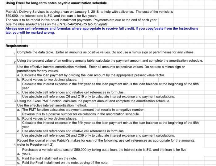

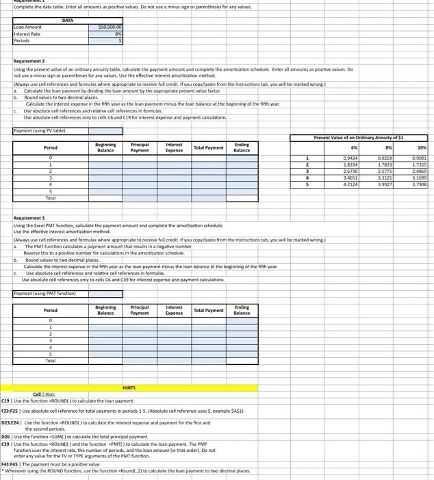
Using Excel for long-term notes payable amortization schedule Patrick's Delivery Services is buying a van on January 1, 2018, to help with deliveries. The cost of the vehicle is $50,000, the interest rate is 8%, and the loan is for five years. The van is to be repaid in five equal installment payments. Payments are due at the end of each year. Use the blue shaded areas on the ENTER-ANSWERS tab for inputs. Always use cell references and formulas where appropriate to receive full credit. If you copy/paste from the Instructions tab, you will be marked wrong. 2 Requirements Complete the data table. Enter all amounts as positive values. Do not use a minus sign or parentheses for any values. Using the present value of an ordinary annuity table, calculate the payment amount and complete the amortization schedule. Use the effective interest amortization method. Enter all amounts as positive values. Do not use a minus sign or parentheses for any values. a. Calculate the loan payment by dividing the loan amount by the appropriate present value factor. b. Round values to two decimal places. Calculate the interest expense in the fifth year as the loan payment minus the loan balance at the beginning of the fifth year. c. Use absolute cell references and relative cell references in formulas. Use absolute cell references C6 and C19 only to calculate interest expense and payment calculations. 3 Using the Excel PMT function, calculate the payment amount and complete the amortization schedule. Use the effective interest amortization method. a. The PMT function calculates a payment amount that results in a negative number. Reverse this to a positive number for calculations in the amortization schedule. b. Round values to two decimal places. Calculate the interest expense in the fifth year as the loan payment minus the loan balance at the beginning of the fifth year. c Use absolute cell references and relative cell references in formulas. Use absolute cell references C6 and C39 only to calculate interest expense and payment calculations. Record the journal entries Patrick's makes for each of the following use cell references as appropriate for the amounts. 4 (refer to Requirement 2) Purchased a vehicle with a cost of $50,000 by taking out a loan, the interest rate is 8%, and the loan is for five a. years. b. Paid the first installment on the note. c. Paid the Final installment on the note, paying off the note. Complete the data Table Enterall amounts as positive values. Do not use a minus signor parentheses for any values DATA Loan Amount Interest Rate Periods $50,000.00 8% 5 Requirement 2 Using the present value of an ordinary annuity table, calculate the payment amount and complete the amortization schedule. Enter all amounts as positive values. Do not use a minus signor parentheses for any values. Use the effective interest amortization method Always use cell references and formulas where appropriate to receive full credit. If you copy/paste from the instructions tabou will be marked wrong) a Calculate the loan payment by dividing the loan amount by the appropriate present value factor Round values to two decimal places Calculate the interest expense in the fifth year as the loan payment minus the loan balance at the beginning of the the year Use absolute cell references and relative cell references in formulas Use absolute cell references only to cells and C19 for interest expense and payment calculations b Payment using PV table) Present Value of 2 Ordinary Annuity of $1 Period Beginning Balance Principal Payment Interest Expense Total Payment Ending Ralance 6% 101 0 1 2 3 4 5 Total 1 2 3 4 5 0.9434 1.8334 2.6730 3.4551 4.2124 0.9.25 1730 25771 3312 3.0927 0.901 17355 2.4869 3.1699 Requirement) Using the Excel PMT function calculate the payment amount and complete the amortization schedule Use the effective interest amortization method (Always use cell references and formulas where appropriate to receive full credit. If you copy/paste from the instructions tab, you will be marked wrong) The PMT function calculates a payment amount that results in a negative numbet Reverse this to a positive number for calculations in the amortisation schedule b Round values to two decimal places Calculate the interest expens in the fifth year as the loan payment minus the loan balance at the beginning of the fifth year Use absolute cel references and relative cell references informas Use absolute cell references only to celk 6 and 9 for interest expense and payment calculations Payment using function Period Beginning Balance Principal Payment Interest Expense Total Payment Ending Balance 0 1 2 3 4 5 Total HINTS Cell Mint C19 Use the function ROUNDE) to calculate the loan payment F23.525 I Use absolute cell reference for total payments in periods 1-5. (Absolute cell reference uses S, example SA$11 023.24 Use the function ROUND) to calculate the interest expense and payment for the first and the second periods 026 Use the function SUM) to calculate the total principal payment C39 Use the function ROUNDC) and the function PMT) to calculate the loan payment. The PMT function uses the interest rate, the number of period, and the loan amount in that order). Do not unter any value for the For TYPE arguments of the PMT function F41.545 The payment must be a positive value Whenever using the ROUND function, use the function Round 21 to calculate the loan payment to two decimal places