MANAGERIAL ECONOMICS

In a Nutshell

In this part you are going to jot down what you have learned BELOW. The said statement of yours could be in a form of concluding statements, arguments, or perspective you have drawn from this lesson. The first two is done for you.

1.Production refers to the transformation of inputs (economic resources) to outputs (products) and can be analyze with the use of a production function which is a mathematical representation of the firm's production activity.

2.Production can be analyze base on its short-run or long-run conditions. Short-run is a time period where a firm is using at least a single fixed input. In this case the Law of Diminishing of Marginal Returns is observed. Stages of production is also determined which illustrates the returns to a factor (increasing or decreasing) of the firm.

Now it's your turn!

3.

4.

5.

REFERENCE:

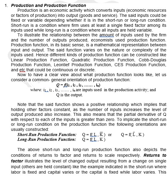
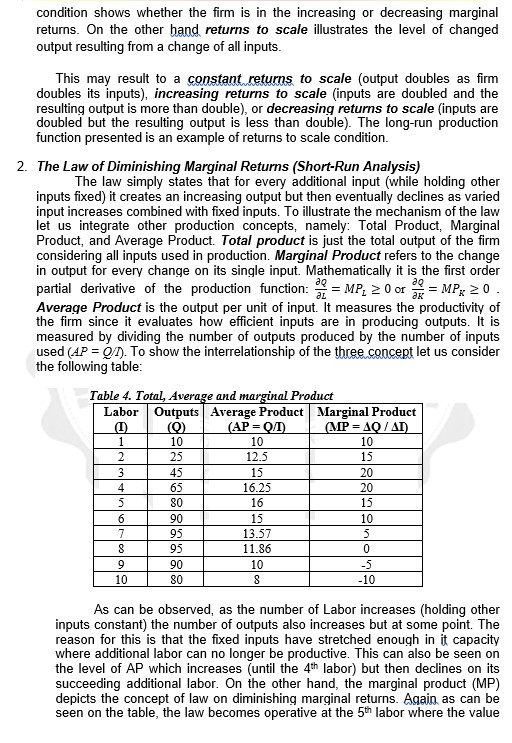
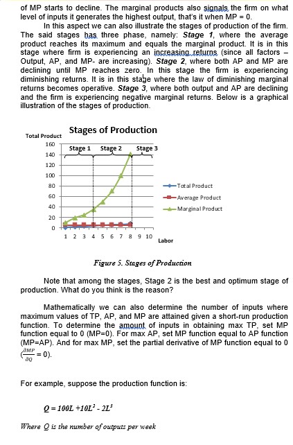
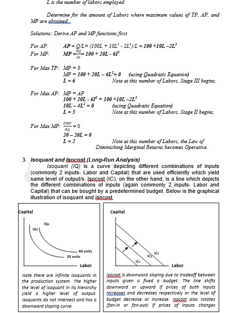
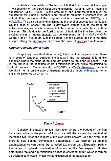
1. Production and Production Function Production is an economic activity which converts inputs (economic resources or factors of production) into output (goods and service). The said inputs could be fixed or variable depending whether it is in the short-run or long-run condition. Short-run is a condition where firm uses at least a single fixed factor among its inputs used while long-run is a condition where all inputs are held variable. To illustrate the relationship between the amount of inputs used by the firm and the number of outputs produced, economists used production function. Production function, in its basic sense, is a mathematical representation between input and output. The said function varies on the nature or complexity of the inputs used. Hence different kinds of production function can be constructed like Linear Production Function, Quadratic Production Function, Cobb-Douglas Production Function, Leontief Production Function, CES Production Function, and etc that could be continuous or discrete. Now to have a clear view about what production function looks like, let us consider a common- general orientation of production function: Q =flil , 12 , is, ...... ; in) where: 11 12 , 13 , ...... . in are inputs used in the production activity; and Q is the output. Note that the said function shows a positive relationship which implies that holding other factors constant, as the number of inputs increases the level of output produced also increase. This also means that the partial derivative of Q with respect to each of the inputs is greater than zero. To implicate the short-run or long-run condition on the production function the following orientations are usually constructed: Short-Run Production Function: Q =f(L , K ) or Q = f(L , K ) Long-Run Production Function: Q = [LL , K ) The above short-run and long-run production function also depicts the conditions of returns to factor and returns to scale respectively. Returns to factor illustrates the level of changed output resulting from a change on single input (others are held constant) like the example indicated in the short-run where labor is fixed and capital varies or the capital is fixed while labor varies. Thiscondition shows whether the firm is in the increasing or decreasing marginal returns. On the other hand returns to scale illustrates the level of changed output resulting from a change of all inputs. This may result to a constant returns to scale (output doubles as firm doubles its inputs), increasing returns to scale (inputs are doubled and the resulting output is more than double), or decreasing returns to scale (inputs are doubled but the resulting output is less than double). The long-run production function presented is an example of returns to scale condition. 2. The Law of Diminishing Marginal Returns (Short-Run Analysis) The law simply states that for every additional input (while holding other inputs fixed) it creates an increasing output but then eventually declines as varied input increases combined with fixed inputs. To illustrate the mechanism of the law let us integrate other production concepts, namely: Total Product, Marginal Product, and Average Product. Total product is just the total output of the firm considering all inputs used in production. Marginal Product refers to the change in output for every change on its single input. Mathematically it is the first order partial derivative of the production function: # = MP, 2 0 or ag = 30 = MP, 20. Average Product is the output per unit of input. It measures the productivity of the firm since it evaluates how efficient inputs are in producing outputs. It is measured by dividing the number of outputs produced by the number of inputs used (AP = 07). To show the interrelationship of the three concept let us consider the following table: Table 4. Total, Average and marginal Product Outputs Average Product Marginal Product (0) (AP = Q/D) (MP = AQ / AI 10 10 10 25 12.5 15 45 15 20 65 16.25 20 30 16 15 90 15 10 95 13.57 5 11.86 0 10 -5 80 8 10 As can be observed, as the number of Labor increases (holding other inputs constant) the number of outputs also increases but at some point. The reason for this is that the fixed inputs have stretched enough in it capacity where additional labor can no longer be productive. This can also be seen on the level of AP which increases (until the 4" labor) but then declines on its succeeding additional labor. On the other hand, the marginal product (MP) depicts the concept of law on diminishing marginal returns. Again as can be seen on the table, the law becomes operative at the 5" labor where the valueof MP starts to decline. The marginal products also signals the firm on what level of inputs it generates the highest output, that's it when MP = 0. In this aspect we can also illustrate the stages of production of the firm. The said stages has three phase, namely: Stage 1, where the average product reaches its maximum and equals the marginal product. It is in this stage where firm is experiencing an increasing returns (since all factors - Output, AP, and MP- are increasing). Stage 2, where both AP and MP are declining until MP reaches zero. In this stage the firm is experiencing diminishing returns. It is in this stage where the law of diminishing marginal returns becomes operative. Stage 3, where both output and AP are declining and the firm is experiencing negative marginal returns. Below is a graphical illustration of the stages of production. Stages of Production Total Product 160 Stage 1 Stage 2 Stage 3 140 120 100 80 Total Product 60 Average Product 40 - Marginal Product 20 0 1 2 3 4 5 6 7 8 9 10 Labor Figure 5. Stages of Production Note that among the stages, Stage 2 is the best and optimum stage of production. What do you think is the reason? Mathematically we can also determine the number of inputs where maximum values of TP, AP, and MP are attained given a short-run production function. To determine the amount of inputs in obtaining max TP, set MP function equal to 0 (MP=0). For max AP, set MP function equal to AP function (MP=AP). And for max MP, set the partial derivative of MP function equal to 0 - = 0). ao For example, suppose the production function is: Q = 1001 +101' - 21' Where O is the number of outputs per weekI is the number of labors employed Determine for the amount of Labors where maximum values of TP. AP, and MP are obtained. Solutions: Derive AP and MP functions first For AP: AP = OL= (1001 + 101' - 20')/I = 100 +10L -21' For MP: MP = = 100 + 20L - 61 For Max TP: MP = 0 MP = 100 + 201 - 61 =0 (using Quadratic Equation) L=6 Note at this number of Labors, Stage III begins. For Max AP: MP = AP 100 + 201 - 61 = 100 +101 -213 10L - 4L' = 0 (using Quadratic Equation) 1=3 Note at this number of Labors, Stage II begins. For Max MP. OMP -= 0 20 - 201 = 0 L =2 Note at this number of Labors, the Law of Diminishing Marginal Returns becomes Operative. 3. Isoquant and (socost (Long-Run Analysis) (soquant (/Q) is a curve depicting different combinations of inputs (commonly 2 inputs- Labor and Capital) that are used efficiently which yield same level of output/s. Isocost (IC), on the other hand, is a line which depicts the different combinations of inputs (again commonly 2 inputs- Labor and Capital) that can be bought by a predetermined budget. Below is the graphical illustration of isoquant and isocost Capital Capital 102 . 40 units 20 units Labor Labor Note there are infinite isoquants in socost is downward sloping due to tradeoff between the production system. The higher inputs given o fixed a budget. The line shifts the level of isoquant in its hierarchy downword or upward if prices of both inputs yield o higher level of output. increases and decreases respectively or the level of Isoquants do not intersect and hos a budget decrease or increase. (socost olso rotates downward sloping curve. (fon-in or fon-out) if prices of inputs changesNotable characteristic of the isoquant is that it is convex at the origin. The convexity of the curve illustrates diminishing marginal rate of technical substitution (MRTS). MRTS is the amount of one input factor that must be substituted for 1 unit of another input factor to maintain a constant level of output. It is the slope of the isoquant and is expressed as: MRTSxy = - MP:/MPx. The said value is diminishing as the level of substitution increases. On the case of isocost the line is downward sloping due to the trade-off between inputs, like which is favorable to have more on a particular input than the other. This is due to the fixed amount of budget the firm has given the existing prices of inputs. (socost can be expressed as: B = QxPx + QvPy where X and Y are inputs, Q is the output, B is the budget, and P is the price of input. Using the function we can derive the slope of isocost equal to -Py/Pv. Optimal Combination of Input Graphically (see illustration below), this condition happens when there is a point of tangency between the isoquant and the isocost It is in this condition where the slope of the isoquant equals to the slope of isocost That is, the firm is in the condition where it minimizes its cost while maximizing its output produced. Mathematically, -MP /MPy = -Py/P- Rewriting the said identity in terms on the ratio of marginal product of input with respect to its price, we have: MP /Px = MPwPy Capital The Optimal Combination of Input [the point of tangency between Isoquant and IC Labor Figure 7. Isopost Consider the next graphical illustration where the budget of the firm increases twice (while prices of inputs are still the same). As the budget increases two times the isocost curve also shifts upward. And for every shift there is new optimal combination determined. If we connect all optimal combinations we can derive the so-called expansion path. Expansion path is the series of optimal combination of inputs as the firm expands. It also determines the long-run relationship between costsand output which is termed as economies of scale (which will be discussed in the next lesson).Capital Expansion Path C1 Labor Figure 8. Optimal Combination and Expansion Park