MATLAB Code
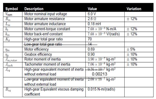
clear all; clc; Vnom=6; Rm=2.6; Lm=0.18e-3; kt=7.68e-3; km=7.68e-3; Kg=70; nm=0.69; ng=0.9; Jmrotor=3.9e-7; Jtach=7.06e-8; Jeq=0.00213; Beq=0.015;
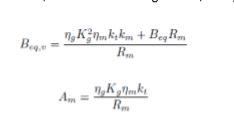
Beqv=((ng*(Kg^2)*nm*kt*km)+(Beq*Rm))/Rm; Am=(ng*Kg*nm*kt)/Rm;
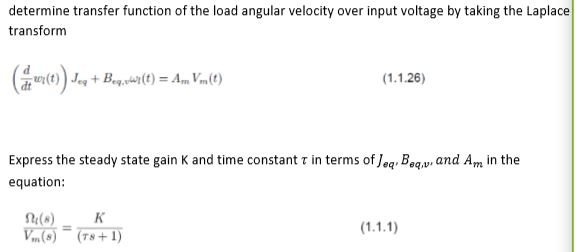
K=Am/Beqv; T=Jeq/Beqv;
--------
Equations:

Answer: Beqv = .0844(N s/rad); Am=.129(N m/V)

Answer: K = 1.528; tau=.0253
----ACTUAL QUESTION----

Symbol Description Value 6.0 V 2.6 0.18 mH Variation Motor nominal input voltage Motor armature resistance Motor armature inductance Motor current-torque constant Motor back-emf constant nom 12% 768 x 10-3 V/(rad/s) 70 | 12% KHigh-gear total gear ratio tio Motor efficiency Geabox efficiency Rotor moment of inertia lachometer moment of inertia High-gear equivalent moment of inerta without external load 0.69 0.90 .90 x 10 kg-m 7.06 x 10 -kg-mT-TT 10% 5% -10% + 10% Trn rit m.rotor eq kg-m 0.00213 without external load High-gear Equivalent viscous damping 0015 N-m/(rad/s) coefficient eq determine transfer function of the load angular velocity over input voltage by taking the Laplace transform + B Express the steady state gain K and time constant equation: r in terms of Jea. Baq,v and Am in the (a) K 1) Create the transfer function, called P using equation 1.1.1. above. Use num, den, and tf as in previous lab 2) Generate and plot angular velocity time response, wi(t), with step input of 5V, for t 0:.01:0.75]. Here is a sample code: t-[0:.01:.51; vn5 *stepfun(t, 0) ; VI-Vm omega_1-lsim (P,vm, t); plot (t, omega_1), grid, title'Omega 1' ylabel ('rad/sec, xlabel ('Time (sec)',shg pause tcreate step function vector with amp 5 change vm from row t vector for later math 3imulate step response using 131m wait for user to hit return before continue 3) Calculate and plot the angular load position (t) = fun(t)dt. One way to do this is to cascade 1/s to the transfer function P in (1). First define integrator transfer function as tf[1, [1 01). Follow similar steps using isim to generate 1(t) 4) Calculate and plot the motor angular velocity com(t) and position ,n(t), using Eq. (1.1.15) How do they compare to the load velocity and position in (2) and (3)? 5) Calculate and plot motor current Im (t) (using Eq, 1.1.5). Explain behavior 6) Calculate and plot back emf voltage ep(t) (using Eq. 1.1.2). Explain behavior 7) Calculate and plot motor torque Tm(t) (using Eq. 1.1.21). Explain behavior 8) Plot motor toque vs. angular velocity using results from (4) and (7). This is known as torque curve. What are the stall torque and no-load velocity? (Tip: need to extrapolate line manually to cross x-axis to determine m_noload) Symbol Description Value 6.0 V 2.6 0.18 mH Variation Motor nominal input voltage Motor armature resistance Motor armature inductance Motor current-torque constant Motor back-emf constant nom 12% 768 x 10-3 V/(rad/s) 70 | 12% KHigh-gear total gear ratio tio Motor efficiency Geabox efficiency Rotor moment of inertia lachometer moment of inertia High-gear equivalent moment of inerta without external load 0.69 0.90 .90 x 10 kg-m 7.06 x 10 -kg-mT-TT 10% 5% -10% + 10% Trn rit m.rotor eq kg-m 0.00213 without external load High-gear Equivalent viscous damping 0015 N-m/(rad/s) coefficient eq determine transfer function of the load angular velocity over input voltage by taking the Laplace transform + B Express the steady state gain K and time constant equation: r in terms of Jea. Baq,v and Am in the (a) K 1) Create the transfer function, called P using equation 1.1.1. above. Use num, den, and tf as in previous lab 2) Generate and plot angular velocity time response, wi(t), with step input of 5V, for t 0:.01:0.75]. Here is a sample code: t-[0:.01:.51; vn5 *stepfun(t, 0) ; VI-Vm omega_1-lsim (P,vm, t); plot (t, omega_1), grid, title'Omega 1' ylabel ('rad/sec, xlabel ('Time (sec)',shg pause tcreate step function vector with amp 5 change vm from row t vector for later math 3imulate step response using 131m wait for user to hit return before continue 3) Calculate and plot the angular load position (t) = fun(t)dt. One way to do this is to cascade 1/s to the transfer function P in (1). First define integrator transfer function as tf[1, [1 01). Follow similar steps using isim to generate 1(t) 4) Calculate and plot the motor angular velocity com(t) and position ,n(t), using Eq. (1.1.15) How do they compare to the load velocity and position in (2) and (3)? 5) Calculate and plot motor current Im (t) (using Eq, 1.1.5). Explain behavior 6) Calculate and plot back emf voltage ep(t) (using Eq. 1.1.2). Explain behavior 7) Calculate and plot motor torque Tm(t) (using Eq. 1.1.21). Explain behavior 8) Plot motor toque vs. angular velocity using results from (4) and (7). This is known as torque curve. What are the stall torque and no-load velocity? (Tip: need to extrapolate line manually to cross x-axis to determine m_noload)
