MATLAB CODE for above mentioned task

I am getting errors in the area marked in bold.

clear all; clc; close all;

%% Define all coefficients for the 4-element Windkessel Model

h = 0.01; % time step

cycles = 10; % number of cycles

beats_min = 72; % number of heart beats in a min

t_beat = 60/beats_min; % duration of a heart beat in seconds

q0 = 500; % average flow rate

t_sys = (2/5)*t_beat; % period of systole in seconds

Tmax =cycles.*t_beat; % Total time of simulation

tT = [0:h:Tmax]; % time vector

% create the inlet flow waveform, originating from the aortic valve

for i=1:length(tT)

Q(i) = fun_Q(tT(i),t_beat,t_sys,q0); %making the inlet flow using fun_Q function

end

% plot blood flow rate over the 10 cycles

figure

plot(tT,Q)

title('Inlet Flow')

set(gca,'FontSize',16)

xlabel( 'Time(s)','FontSize',20,'Interpreter','latex')

ylabel('Flowrate (ml/s)','FontSize',20,'Interpreter','latex')

r = 0.5; %mmHg-s/mL

L = 0.005; %mmHg-s^2/mL

C = 1.22; %mL/mmHg

R = 0.79; %mmHg-s/mL

%% %%%%%%%%%%%%%%%%%%%%%%%% Explicit Euler %%%%%%%%%%%%%%%%%%%%%%%%%%

%% solve for the distal pressure, Pd

t(1) = 0; % initial values for t and Pd

Pd(1) = 80;

dt = h;

% Time marching to find next values of Pd by solving ODE using Explicit Euler method

for i = 1:Tmax/dt

Pd(i+1)= (1-(h/(R.*C))).*Pd(i) + h.*(Q(i)/C);

t(i+1)= t(i) + 1;

end

%% solve for the flow rate through the inductor, QL

QL(1)= 0; % initial value of QL

% Time marching to find next values of QL by solving ODE using Explicit Euler method

for i=1:Tmax/dt

QL(i+1)=(1-(h.*r)/L).*QL(i) + (Q(i).*(h.*r))/L ;

t(i+1)= t(i) + 1;

end

%% Pressure

Qr = Q(t) - QL(t); % find Qr and Pressure using the element relations. Error: Array indices must be positive integers or logical values. Error in test_bioe (line 58) Qr = Q(t) - QL(t); % find Qr and Pressure using the element relations

P = Pd(t) + r.*Qr;

figure

plot(t,P)

title('Pressure Explicit')

set(gca,'FontSize',16)

xlabel( 'Time(s)','FontSize',20,'Interpreter','latex')

ylabel('Arterial pressure (mm Hg)','FontSize',20,'Interpreter','latex')

%% %%%%%%%%%%%%%%%%%%%%%%%%%% Implicit Euler %%%%%%%%%%%%%%%%%%%%%%%%%%%%%%%%

%% solve for the distal pressure, Pd

Pd(1) = 80 ; % initial values for Pd

t(1) = 0;

% Time marching to find next values of Pd by solving ODE using Implicit Euler method

for i=1:Tmax/dt

Pd(i+1) = (Pd(i) + (Q(n+1).*h)/C)/ (1 + (h / (R.*C))) ;

t(i+1)= t(i) + 1;

end

%% solve for the flow rate through the inductor, QL

QL(1) = 0; % initial values for QL

% Time marching to find next values of QL by solving ODE using Implicit Euler method

for i=1:Tmax/dt

QL(i+1) = (QL(i) + (h.*r).*(Q(i+1)))/ (1 + (h / (r.*L))) ;

t(i+1)= t(i) + 1;

end

%% Pressure

Qr = Q(t) - QL(t); % find Qr and Pressure using the element relations

P = Pd(t) + r.*Qr;

figure

plot(t,P)

title('Pressure Implicit')

set(gca,'FontSize',16)

xlabel( 'Time(s)','FontSize',20,'Interpreter','latex')

ylabel('Arterial pressure (mm Hg)','FontSize',20,'Interpreter','latex')

%% %%%%%%%%%%%%%%%%%%%%%%%%% Runge-Kutta 4th order %%%%%%%%%%%%%%%%%%%%%%%%%%

%% solve for Pd

f=@(x,y) (h/C).*(Q(t) - Pd(t)/R); %define the handle function for Pd equation

Pd(1) = 80 ; % initial values for Pd

t(1) = 0;

% Find each one of Runge-Kutta constants at each time point and march through time

for i=1:Tmax/dt

K1= (h/C).*(Q(t(i)) - Pd(t(i))/R) ;

K2= (h/C).*(Q(t(i)+h/2) - Pd(t(i))/R +K1/2);

K3= (h/C).*(Q(t(i)+h/2) - Pd(t(i))/R +K2/2);

K4= (h/C).*(Q(t(i)+h) - Pd(t(i))/R +K3);

Pd(i+1)= Pd(1) + (1/6).*(K1 + 2.*K2 + 2.*K3 + K4 );

t(i+1)= t(i) +1;

end

%% Solve for QL

g=@(x,y) (r/L).*(Q(t) - QL(t)); %define the handle function for QL

QL(1) = 0; %initial values for QL and time

t(1) = 0;

for i=1:Tmax/dt % Find each one of Runge-Kutta constants at each time point and march time

K1 = h.*(r/L).*(Q(i)-QL(i));

K2 = h.*(r/L).*(Q(i+h/2)-(QL(i)+K1/2));

K3 = h.*(r/L).*(Q(i+h/2)-(QL(i)+K2/2));

K4 = h.*(r/L).*(Q(i+1)-(QL(i)+K3));

QL(i+1) = QL(i) + (1/6).*(K1 + 2.*K2 + 2.*K3 + k4);

t(i+1) = t(i)+1;

end

%% Pressure

Qr = Q(t) - QL(t); % find Qr and Pressure using the element relations

P = Pd(t) + r.*Qr;

figure

plot(t,P)

title('Pressure RK4')

set(gca,'FontSize',16)

xlabel( 'Time(s)','FontSize',20,'Interpreter','latex')

ylabel('Arterial pressure (mm Hg)','FontSize',20,'Interpreter','latex')

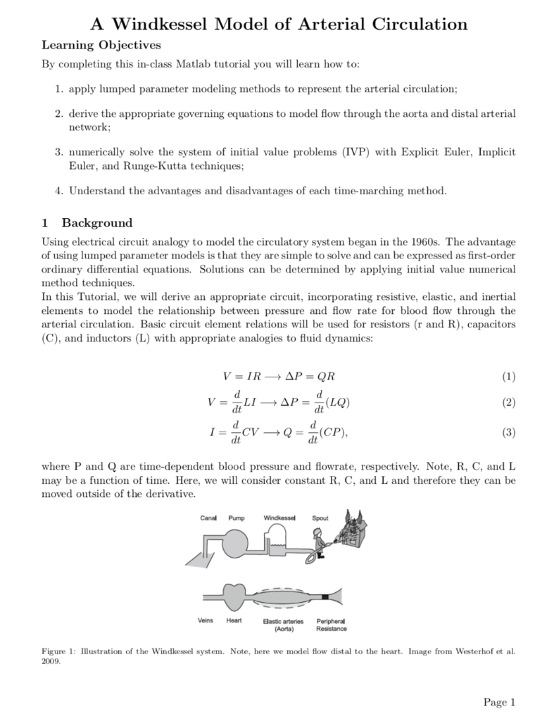
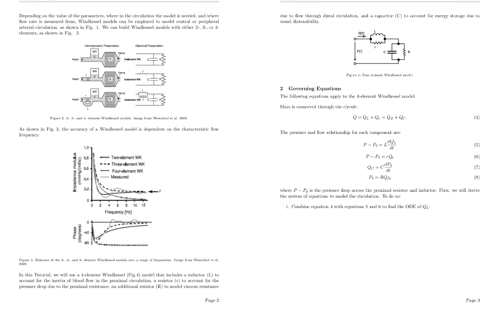
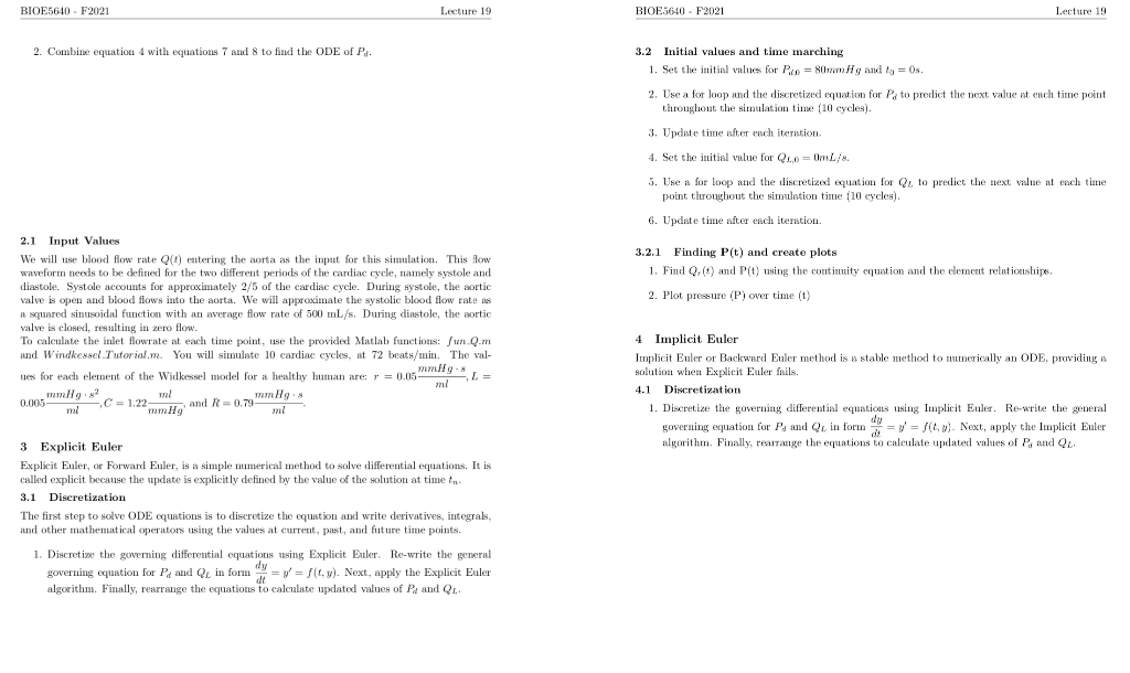
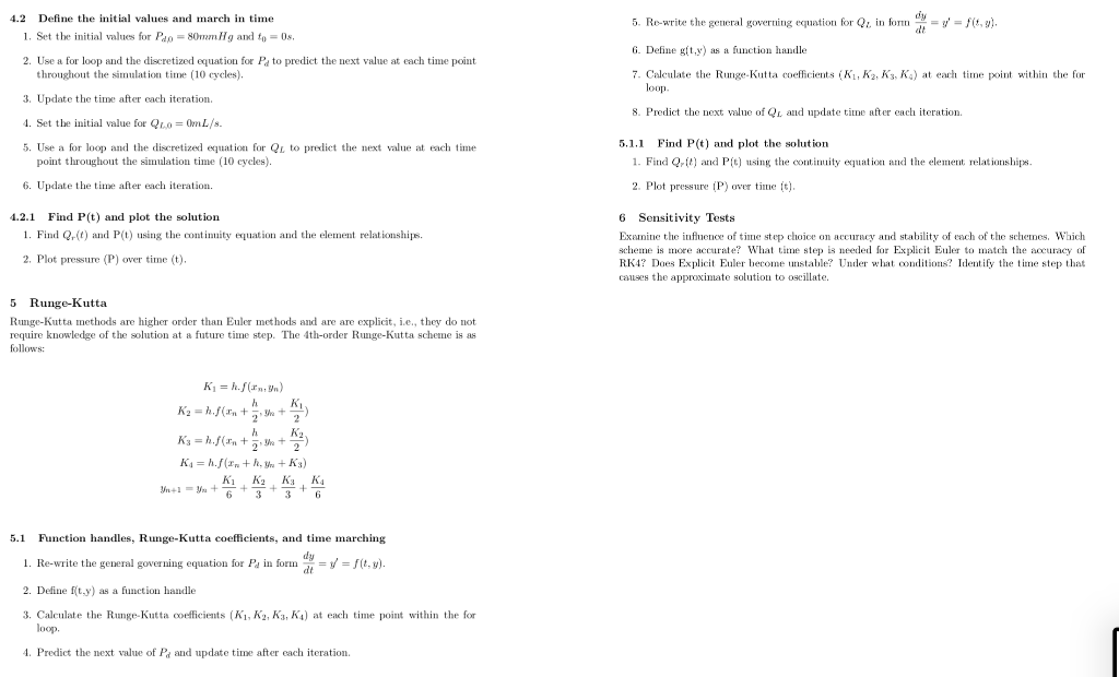
A Windkessel Model of Arterial Circulation Learning Objectives By completing this in-class Matlab tutorial you will learn how to: 1. apply lumped parameter modeling methods to represent the arterial circulation; 2. derive the appropriate governing equations to model flow through the aorta and distal arterial network; 3. numerically solve the system of initial value problems (IVP) with Explicit Euler, Implicit Euler, and Runge-Kutta techniques; 4. Understand the advantages and disadvantages of each time-marching method. 1 Background Using electrical circuit analogy to model the circulatory system began in the 1960s. The advantage of using lumped parameter models is that they are simple to solve and can be expressed as first-order ordinary differential equations. Solutions can be determined by applying initial value numerical method techniques. In this Tutorial, we will derive an appropriate circuit, incorporating resistive, elastic, and inertial elements to model the relationship between pressure and flow rate for blood flow through the arterial circulation. Basic circuit element relations will be used for resistors ( r and R), capacitors (C), and inductors (L) with appropriate analogies to fluid dynamics: V=IRP=QRV=dtdLIP=dtd(LQ)I=dtdCVQ=dtd(CP), where P and Q are time-dependent blood pressure and flowrate, respectively. Note, R,C, and L may be a function of time. Here, we will consider constant R, C, and L and therefore they can be moved outside of the derivative. Figure 1: Illustration of the Windkessel system. Note, here we model flow distal to the heart. Image from Westerhof et al. 2009. Depending on the value of the paraneters, where in the circulation the model is needed, and where due to flow through distal circulation, and a caparit (C) to anount for energy storage due to flow rate is measured from, Windkessel models can be employed to model central or peripheral vessel distensibility. arterial circulation, as shown in Fig. 1. We can build Windkessel models with either 2-, 3-, ar 4elements, as shown in Fig. 2. Pigure 4i Four element bindkesced motel 2 Governing Equations The following equations apply to the 4-elenent Windkrsed model. Mass is conserved through the circuit: Fagurn 2: 2, st, and 4- rement Windlorworl mockels. Imagy from Westerhaf ent al. avod. Q=QL+Qr=QR+QC. As shown in Fig. 3, the accuracy of a Windkeseel model is dependent on the characteristic flow The presstare and flow relationahip for each component are: frequency. PPd=LdtdQsPPd=rQrQC=CdtdPaPd=RQR where PPd is the pressure drop across the proximal resistor and inductor. First, we will derive the system of equations to model the circulation. To do sor 1. Combine equation 4 with equations 5 and 6 to find the ODE of Qz. In this Tutorial, we will use a 4-element Windkessel (Fig.4) moxlel that includes a inductor (L) to account for the inertia of blood flow in the proximal circulation, a resistor ( r ) to acoount for the pressure drop due to the proximal resistance, an additional resistor (R) to model viscons resistance Page 2 Page 3 2. Combine equation 4 with equations 7 and 8 to find the ODE of Pd. 3.2 Initial values and time marching 1. Set the initial values for Pa0=80manHg and t0=0 s. 2. Use a for loop and the discretized equation for Pd to predict the next value at ench time point throughout the simulation time (10 cycles). 3. Update time after each iteration. 4. Set the initial value for QL,0=0mL/s. 5. Use a for loop and the discretized equation for QL to predict the next value at each time point throughout the simulation time (10 cycles). 6. Update time after each iteration. 2.1 Input Values 3.2.1 Finding P(t) and create plots We will use blood flow rate Q(t) entering the aorta as the input for this simulation. This flow 1. Find Q,(t) and P(t) using the continuity equation and the element relutionships. diastole. Systole accounts for approximately 2/5 of the cardiac cycle. During systole, the aortic 2. Plot pressure (P) over time ( t) valve is open and blood flows into the aorta. We will approximate the systolic blood flow rate as a squared sinusoidal function with an average flow rate of 500mL/s. During diastole, the aortic valve is closed, resulting in zero flow. To calculate the inlet flowrate at each time point, use the provided Matlab functions: Jun.Q.m 4 Implicit Euler and Windkessel.Tutorial.m. You will simulate 10 cardiac cycles, at 72 beats /min. The valImplicit Euler or Backward Euler method is a stable method to mumerically an ODE, providing a ues for each element of the Widkessel model for a healthy human are: r=0.05mlmmHg8,L= solution when Explicit Euler fails. 0,005mlmmHgs2,C=1.22mmHgml, and R=0.79mlmmHgs. 4.1 Discretization 1. Discretize the governing differential equations using Implicit Euler. Re-write the general governing equation for Pd and QL in form dtdy=y=f(t,y). Next, apply the Implicit Euler 3 Explicit Euler algorithm. Finally, rearrange the equations to calculate updated values of Pof and QL. Explicit Euler, or Forward Euler, is a simple numerical method to solve differential equations. It is called explicit because the update is explicitly defined by the value of the solution at time tn. 3.1 Discretization The first step to solve ODE equations is to discretize the equation and write derivatives, integrals, and other mathematical operators using the values at current, past, and future time points. 1. Discretize the governing differential equations using Explicit Euler. Re-write the general governing equation for Pd and QL in form dtdy=y=f(t,y). Next, apply the Explicit Euler algorithm. Finally, rearrange the equations to calculate updated values of Pd and QL. 4.2 Define the initial values and march in time 5. Re-write the general governing equation for QL in form dtdy=y=f(t,y). 1. Set the initial values for Pd=80mmHg and t0=0s. 6. Define g(t,y) as a function handle 2. Use a for loop and the discretized equation for Pd to predict the next value at each time point 7. Calculate the Runge-Kutta coefficients (K1,K2,K3,K4) at each time point within the for throughout the simulation time (10 cycles). loop. 3. Update the time after each iteration. 8. Predict the next value of QL and update time after each iteration. 4. Set the initial value for QL,0=0mL/s. 5.1.1 Find P(t) and plot the solution 5. Use a for loop and the discretized equation for QL to predict the next value at each time 1. Find Qr(t) and P(t) using the continuity equation and the element relationships. 6. Update the time after each iteration. 2. Plot pressure ( P) over time (t). 4.2.1 Find P(t) and plot the solution 6 Sensitivity Tests 1. Find Qr(t) and P(t) using the continuity equation and the element relationships. Examine the influenoe of time step choice on accuracy and stability of each of the schemes, Which 2. Plot pressure (P) over time ( t). scheme is more accurate? What time step is needed for Explicit Euler to match the aocuracy of RK4? Does Explicit Euler become unstable? Under what conditions? Identify the time step that canses the approximate solution to oscillate. 5 Runge-Kutta Runge-Kutta methods are higher order than Euler methods and are are explicit, i.e., they do not require knowledge of the solution at a future time step. The 4th-order Runge-Kutta scheme is as follows: K1=hf(xn,yn)K2=hf(xn+2h,yn+2K1)K3=hf(xn+2h,yn+2K2)K4=hf(xn+h,yn+K3)yn+1=yn+6K1+3K2+3K3+6K4 5.1 Function handles, Runge-Kutta coefficients, and time marching 1. Re-write the general governing equation for Pd in form dtdy=y=f(t,y). 2. Define f(t,y) as a function handle 3. Calculate the Runge-Kutta coefficients (K1,K2,K3,K4) at each time point within the for loop. 4. Predict the next value of Pd and update time after each iteration