Matlab. (Curve fitting) The temperature dependence of the reaction rate coefficient of a chemical reaction is...
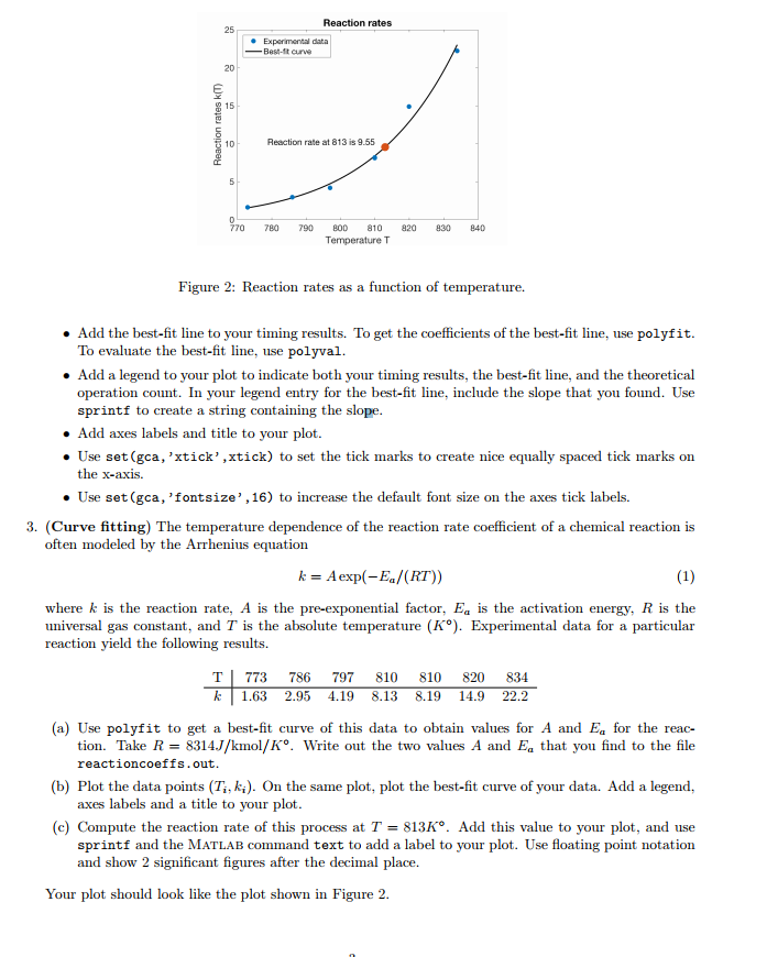
Reaction rates 25 Best-ft curve 20 15 10 Reaction rate at 813 is 9.55 770 780 790 0D 810 820 830 840 Temperature T Figure 2: Reaction rates as a function of temperature. . Add the best-fit line to your timing results. To get the coefficients of the best-fit line, use polyfit. To evaluate the best-fit line, use polyval . Add a legend to your plot to indicate both your timing results, the best-fit line, and the theoretical operation count. In your legend entry for the best-fit line, include the slope that you found. Use sprintf to create a string containing the slope . Add axes labels and title to your plot. . Use set (gca, 'xtick' ,xtick) to set the tick marks to create nice equally spaced tick marks on the x-axis. . Use set (gca, 'fontsize',16) to increase the default font size on the axes tick labels. 3. (Curve fitting) The temperature dependence of the reaction rate coefficient of a chemical reaction is often modeled by the Arrhenius equation k A exp(-Ea/ (RT)) where k is the reaction rate, A is the pre-exponential factor, Ea is the activation energy, R is the universal gas constant, and T is the absolute temperature (K). Experimental data for a particular reaction yield the following results. T773 786 797 810 810 820 834 k 1.63 2.95 4.19 8.13 8.19 14.9 22.2 (a) Use polyfit to get a best-fit curve of this data to obtain values for A and Ea for the reac- tion. Take R 8314J/kmol/K. Write out the two values A and Ea that you find to the file reactioncoeffs.out (b) Plot the data points (Ti, ki). On the same plot, plot the best-fit curve of your data. Add a legend, axes labels and a title to your plot (c) Compute the reaction rate of this process at T- 813Ko. Add this value to your plot, and use sprintf and the MATLAB command text to add a label to your plot. Use floating point notation and show 2 significant figures after the decimal place Your plot should look like the plot shown in Figure 2. Reaction rates 25 Best-ft curve 20 15 10 Reaction rate at 813 is 9.55 770 780 790 0D 810 820 830 840 Temperature T Figure 2: Reaction rates as a function of temperature. . Add the best-fit line to your timing results. To get the coefficients of the best-fit line, use polyfit. To evaluate the best-fit line, use polyval . Add a legend to your plot to indicate both your timing results, the best-fit line, and the theoretical operation count. In your legend entry for the best-fit line, include the slope that you found. Use sprintf to create a string containing the slope . Add axes labels and title to your plot. . Use set (gca, 'xtick' ,xtick) to set the tick marks to create nice equally spaced tick marks on the x-axis. . Use set (gca, 'fontsize',16) to increase the default font size on the axes tick labels. 3. (Curve fitting) The temperature dependence of the reaction rate coefficient of a chemical reaction is often modeled by the Arrhenius equation k A exp(-Ea/ (RT)) where k is the reaction rate, A is the pre-exponential factor, Ea is the activation energy, R is the universal gas constant, and T is the absolute temperature (K). Experimental data for a particular reaction yield the following results. T773 786 797 810 810 820 834 k 1.63 2.95 4.19 8.13 8.19 14.9 22.2 (a) Use polyfit to get a best-fit curve of this data to obtain values for A and Ea for the reac- tion. Take R 8314J/kmol/K. Write out the two values A and Ea that you find to the file reactioncoeffs.out (b) Plot the data points (Ti, ki). On the same plot, plot the best-fit curve of your data. Add a legend, axes labels and a title to your plot (c) Compute the reaction rate of this process at T- 813Ko. Add this value to your plot, and use sprintf and the MATLAB command text to add a label to your plot. Use floating point notation and show 2 significant figures after the decimal place Your plot should look like the plot shown in Figure 2