MATLAB hw

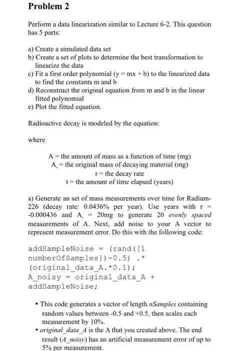
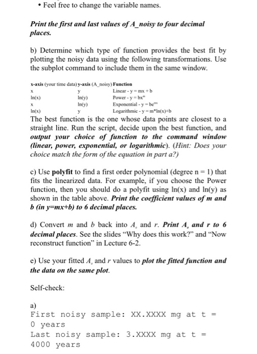
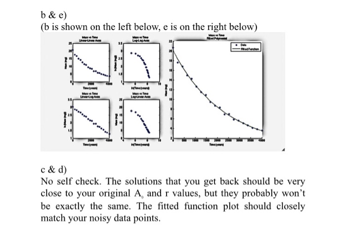
Problem 2 Perform a data linearization similar to Lecture 6-2. This question has 5 parts: a) Create a simulated data set b) Create a set of plots to determine the best transformation to linearize the data c) Fit a first order polynomial (y = mx +b) to the linearized data to find the constants m and b d) Reconstruct the original equation from m and b in the linear fitted polynomial e) Plot the fitted equation. Radioactive decay is modeled by the equation: where A = the amount of mass as a function of time (mg) A = the original mass of decaying material (mg) r= the decay rate t = the amount of time elapsed (years) a) Generate an set of mass measurements over time for Radium- 226 (decay rate: 0.0436% per year). Use years with r = -0.000436 and A = 20mg to generate 20 evenly spaced measurements of A. Next, add noise to your A vector to represent measurement error. Do this with the following code: addSampleNoise = (rand ([1 numberOfSamples])-0.5) .* (original data A.*0.1); A noisy = original_data_A + addSampleNoise; This code generates a vector of length Samples containing random values between -0.5 and +0.5, then scales each measurement by 10%. original_data_A is the A that you created above. The end result (A noisy) has an artificial measurement error of up to 5% per measurement. Feel free to change the variable names. Print the first and last values of A noisy to four decimal places. b) Determine which type of function provides the best fit by plotting the noisy data using the following transformations. Use the subplot command to include them in the same window. x-axis (your time data)y-axis (A_noisy) Function Linear-y=mx+b In(x) In(y) Power-y=bx In(y) Exponential-y-be In(x) Logarithmic - y=min(x)+ The best function is the one whose data points are closest to a straight line. Run the script, decide upon the best function, and output your choice of function to the command window (linear, power, exponential, or logarithmic). (Hint: Does your choice match the form of the equation in part a?) c) Use polyfit to find a first order polynomial (degree n = 1) that fits the linearized data. For example, if you choose the Power function, then you should do a polyfit using In(x) and In(y) as shown in the table above. Print the coefficient values of m and b (in y=mx+b) to 6 decimal places. d) Convert m and b back into A, and r. Print A, and r to 6 decimal places. See the slides "Why does this work?" and "Now reconstruct function in Lecture 6-2. e) Use your fitted A and r values to plot the fitted function and the data on the same plot. Self-check: First noisy sample: XX.XXXX mg at t = 0 years Last noisy sample: 3.XXXX mg at t = 4000 years b&e) (b is shown on the left below, e is on the right below) LALA : : : c& d) No self check. The solutions that you get back should be very close to your original A, and r values, but they probably won't be exactly the same. The fitted function plot should closely match your noisy data points. Problem 2 Perform a data linearization similar to Lecture 6-2. This question has 5 parts: a) Create a simulated data set b) Create a set of plots to determine the best transformation to linearize the data c) Fit a first order polynomial (y = mx +b) to the linearized data to find the constants m and b d) Reconstruct the original equation from m and b in the linear fitted polynomial e) Plot the fitted equation. Radioactive decay is modeled by the equation: where A = the amount of mass as a function of time (mg) A = the original mass of decaying material (mg) r= the decay rate t = the amount of time elapsed (years) a) Generate an set of mass measurements over time for Radium- 226 (decay rate: 0.0436% per year). Use years with r = -0.000436 and A = 20mg to generate 20 evenly spaced measurements of A. Next, add noise to your A vector to represent measurement error. Do this with the following code: addSampleNoise = (rand ([1 numberOfSamples])-0.5) .* (original data A.*0.1); A noisy = original_data_A + addSampleNoise; This code generates a vector of length Samples containing random values between -0.5 and +0.5, then scales each measurement by 10%. original_data_A is the A that you created above. The end result (A noisy) has an artificial measurement error of up to 5% per measurement. Feel free to change the variable names. Print the first and last values of A noisy to four decimal places. b) Determine which type of function provides the best fit by plotting the noisy data using the following transformations. Use the subplot command to include them in the same window. x-axis (your time data)y-axis (A_noisy) Function Linear-y=mx+b In(x) In(y) Power-y=bx In(y) Exponential-y-be In(x) Logarithmic - y=min(x)+ The best function is the one whose data points are closest to a straight line. Run the script, decide upon the best function, and output your choice of function to the command window (linear, power, exponential, or logarithmic). (Hint: Does your choice match the form of the equation in part a?) c) Use polyfit to find a first order polynomial (degree n = 1) that fits the linearized data. For example, if you choose the Power function, then you should do a polyfit using In(x) and In(y) as shown in the table above. Print the coefficient values of m and b (in y=mx+b) to 6 decimal places. d) Convert m and b back into A, and r. Print A, and r to 6 decimal places. See the slides "Why does this work?" and "Now reconstruct function in Lecture 6-2. e) Use your fitted A and r values to plot the fitted function and the data on the same plot. Self-check: First noisy sample: XX.XXXX mg at t = 0 years Last noisy sample: 3.XXXX mg at t = 4000 years b&e) (b is shown on the left below, e is on the right below) LALA : : : c& d) No self check. The solutions that you get back should be very close to your original A, and r values, but they probably won't be exactly the same. The fitted function plot should closely match your noisy data points
