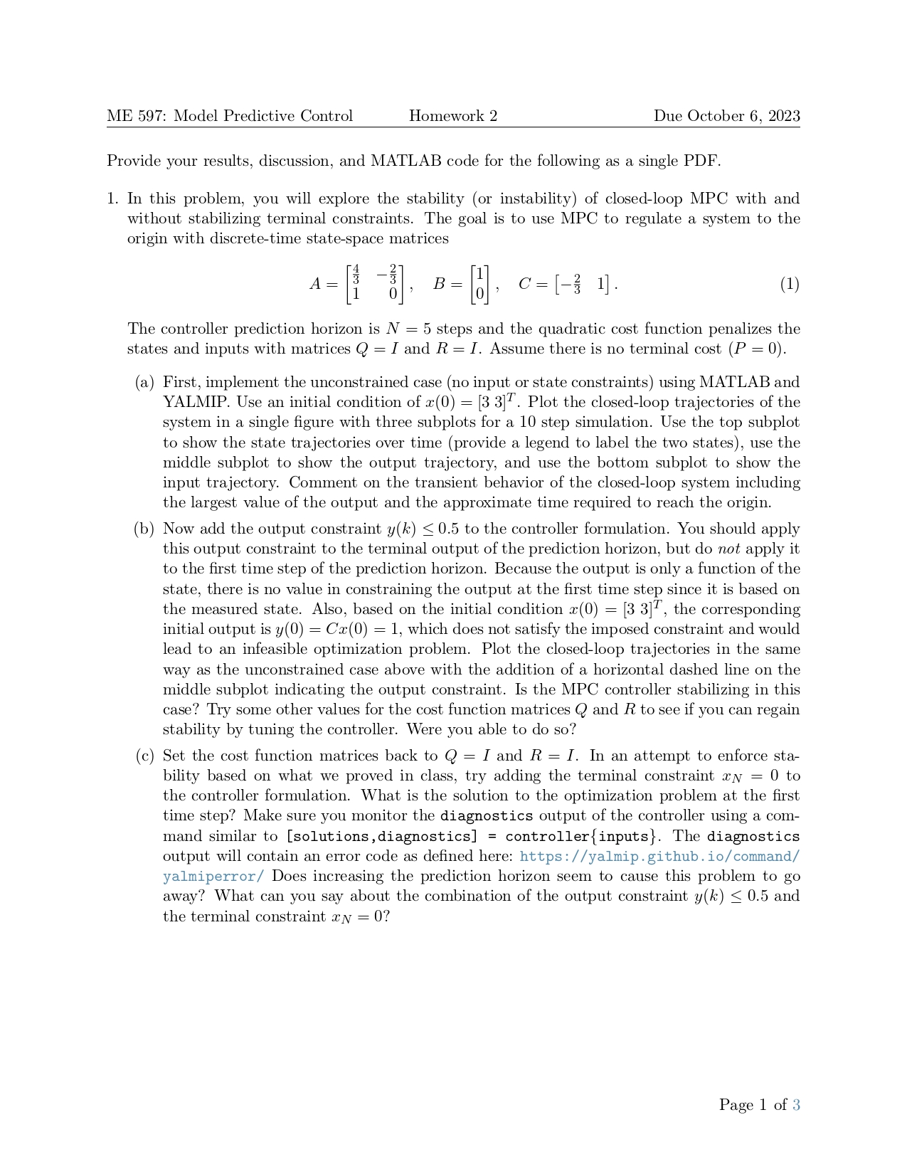
ME 597: Model Predictive Control Homework 2 Due October 6, 2023 Provide your results, discussion, and MATLAB code for the following as a single PDF. 1. In this problem, you will explore the stability (or instability) of closed-loop MPC with and without stabilizing terminal constraints. The goal is to use MPC to regulate a system to the origin with discrete-time state-space matrices A = B = " C = [-1]. " (1) The controller prediction horizon is N = 5 steps and the quadratic cost function penalizes the states and inputs with matrices Q = I and R = I. Assume there is no terminal cost (P = 0). (a) First, implement the unconstrained case (no input or state constraints) using MATLAB and YALMIP. Use an initial condition of x(0) = [33]. Plot the closed-loop trajectories of the system in a single figure with three subplots for a 10 step simulation. Use the top subplot to show the state trajectories over time (provide a legend to label the two states), use the middle subplot to show the output trajectory, and use the bottom subplot to show the input trajectory. Comment on the transient behavior of the closed-loop system including the largest value of the output and the approximate time required to reach the origin. (b) Now add the output constraint y(k) 0.5 to the controller formulation. You should apply this output constraint to the terminal output of the prediction horizon, but do not apply it to the first time step of the prediction horizon. Because the output is only a function of the state, there is no value in constraining the output at the first time step since it is based on the measured state. Also, based on the initial condition x(0) = [33], the corresponding initial output is y(0) = Cx(0) = 1, which does not satisfy the imposed constraint and would lead to an infeasible optimization problem. Plot the closed-loop trajectories in the same way as the unconstrained case above with the addition of a horizontal dashed line on the middle subplot indicating the output constraint. Is the MPC controller stabilizing in this case? Try some other values for the cost function matrices Q and R to see if you can regain stability by tuning the controller. Were you able to do so? = (c) Set the cost function matrices back to Q I and R = I. In an attempt to enforce sta- bility based on what we proved in class, try adding the terminal constraint xN = 0 to the controller formulation. What is the solution to the optimization problem at the first time step? Make sure you monitor the diagnostics output of the controller using a com- mand similar to [solutions, diagnostics] = controller{inputs}. The diagnostics output will contain an error code as defined here: https://yalmip.github.io/command/ yalmiperror/ Does increasing the prediction horizon seem to cause this problem to go away? What can you say about the combination of the output constraint y(k) 0.5 and the terminal constraint xN = 0? Page 1 of 3