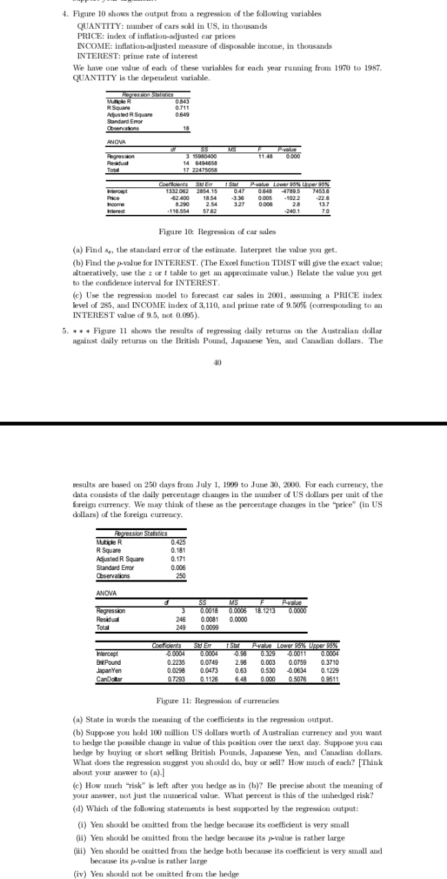
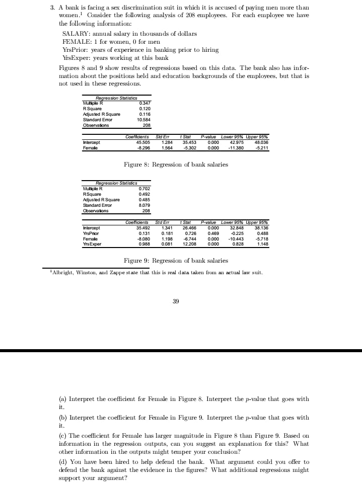
Mechanical components are being produced continuously. A quality control program for the mechanical components requires a close estimate of the proportion defective in production when all settings are correct. 1020 components are examined under these conditions, and 27 of the 1020 items are found to be defective. (a) Find a point estimate of the proportion defective. (b) Find a 95% two-sided confidence interval. (c) Find an upper limit giving 95% level of confidence that the true proportion defective is less than this limiting value.Mechanical components are produced continuously in large numbers on a production line. When the machines are correctly adjusted, extensive data show that the propor- tion of defective components is 0.027. If the proportion of defectives in a sample of size 50 is so large that the result is significant at the 5% level, the production line will be stopped for adjustment. a) What probability distribution applies? b) What is the smallest proportion of defective items in a sample of 50 that will stop the production line?4. Figure 10 shows the output from a regression of the following variables QUANTITY: number of cars sold in US, in thousands PRICE: index of inflation-adjusted car prices INCOME: inflation-adjusted measure of disposable income, in thousands INTEREST: prime rate of interest We have one value of each of these variables for each year running from 1970 to 1987. QUANTITY is the dependent variable. Regression Statistics Mungle R 0.843 R Square 0.711 Adjusted R Square 0.649 Standard Error Observations 18 ANOVA SS MS 15080400 11,48 0:000 Rockdual 14 Total 17 22475058 Confidents f Stat Panlue Lower 95% Upper 95% Intercept 1332.062 2854.15 0.47 0.648 -4789 5 7453.6 Price 62 400 18.54 -3.36 0 00S 102 2 -22.6 #.290 2.54 327 0:006 13.7 Interest -116.554 57 82 -240.1 7.0 Figure 10: Regression of car sales (a) Find se, the standard error of the estimate. Interpret the value you get. (b) Find the p-value for INTEREST. (The Excel function TDIST will give the exact value; udtneratively, use the = or t table to get an approximate value.) Relate the value you get to the confidence interval for INTEREST. (c) Use the regression model to forecast car sales in 2001, assuming a PRICE index level of 285, and INCOME index of 3,110, and prime rate of 9.50% (corresponding to an INTEREST value of 9.5, not 0.095). 5. * * * Figure 11 shows the results of regressing daily returns on the Australian dollar against daily returns on the British Pound, Japanese Yen, and Canadian dollars. The results are based on 250 days from July 1, 1999 to June 30, 2000. For each currency, the data consists of the daily percentage changes in the number of US dollars per unit of the foreign currency. We may think of these as the percentage changes in the "price" (in US dollars) of the foreign currency. Foorossion Statistics Multigle R 0.425 R Square 0.181 Adjusted R Square 0.17 Standard Error 0.006 Observations 250 ANOVA d SS MS P-value Regression 0.0016 0.0006 18.1213 0.0800 Residual 246 0.0081 0.0000 Total 249 0,0099 Copficants Stat Pivalue Lower 95% Upper 95% hiercept -0.000 0.0004 -0.98 0.329 -0.001 0.0004 Brit Pound 0.2235 0.0749 2.98 0.003 0.0759 0.3710 JapanYen 0.0296 0.0473 0.63 0.530 -0.0634 0.1229 CanDollar 0 7293 0.1126 6.48 0.000 0.5076 0.9511 Figure 11: Regression of currencies (a) State in words the meaning of the coefficients in the regression output. (b) Suppose you hold 100 million US dollars worth of Australian currency and you want to hedge the possible change in value of this position over the next day. Suppose you can hedge by buying or short selling British Pounds, Japanese Yen, and Canadian dollars. What does the regression suggest you should do, buy or sell? How much of each? [Think about your answer to (a).] (c) How much "risk" is left after you hedge as in (b)? Be precise about the meaning of your answer, not just the numerical value. What percent is this of the unhedged risk? (d) Which of the following statements is best supported by the regression output: (i) Yen should be omitted from the hedge because its coefficient is very small (i) Yen should be omitted from the hedge because its p-value is rather large (ill) Yen should be omitted from the hedge both because its coefficient is very small and because its p-value is rather large (iv) Yen should not be omitted from the hedge3. A bank is facing a sex discrimination suit in which it is accused of paying men more than women.! Consider the following analysis of 208 employees. For each employee we have the following information: SALARY: annual salary in thousands of dollars FEMALE: 1 for women, 0 for men YrsPrior: years of experience in banking prior to hiring YrsExper: years working at this bank Figures 8 and 9 show results of regressions based on this data. The bank also has infor- mation about the positions held and education backgrounds of the employees, but that is not used in these regressions. Regression Statistics Multiple R 0347 R Square 0.120 Adjusted R Square 0.116 Standard Error 10.584 Observations 208 Coefficients Stat P-valve Lower 95% Upper 95% Intercept 45.50 1.284 35.453 0.000 42.975 18.036 Female -8.296 1564 -5.302 0.000 11.380 -5.211 Figure 8: Regression of bank salaries Regression Statistics Multiple R 0.702 RSquare 0492 Adjusted R Square 0485 Standard Error 4079 Observations 208 Coefficients SId En Stat "-valve Lower 95% Upper 95% Intercept 35.492 1.341 26.466 0.000 32.848 38.136 YrsPrior 0.131 0.181 0.726 0.469 -0.225 0.488 Female 8.080 1.198 -6.744 0.000 10.443 -5.718 Yrs Exper 0.988 0.081 12.208 0.000 0.828 1.148 Figure 9: Regression of bank salaries Albright, Winston, and Zappe state that this is real data taken from an actual law suit. 39 (a) Interpret the coefficient for Female in Figure 8. Interpret the p-value that goes with it. (b) Interpret the coefficient for Female in Figure 9. Interpret the p-value that goes with it. (c) The coefficient for Female has larger magnitude in Figure 8 than Figure 9. Based on information in the regression outputs, can you suggest an explanation for this? What other information in the outputs might temper your conclusion? (d) You have been hired to help defend the bank. What argument could you offer to defend the bank against the evidence in the figures? What additional regressions might support your argument?1. A drugstore chain has collected data on of 50 of its stores. For each store it has values of the following two variables: PROMOTE: Store promotional expenditure as a percentage of expenditure by leading competitor in the store's area SALES: Store sales as a percentage of leading competitor's Figure 6 shows part of the output from a regression of SALES against PROMOTE. ANDVA Regression 2172.88 Residual 18 2624.74 Total 49 Coericants Intercept 25.126 11 883 Promote 0.762 0.121 Figure 6: Drugstore Regression (a) Interpret the coefficient for PROMOTE in words. (b) Find the R- and standard error of the estimate s. (c) Find the t-statistic for PROMOTE. What can you conclude from this value? (d) Find a 95%% confidence interval the coefficient for PROMOTE. 2. Figure 7 shows results of a regression of the US minimum wage during 1950-1994 against time. The time variable is measured in years since 1950 and therefore runs from 0 to 44. The wage variable is in dollars per hour and increased from 0.75 to 4.25 over this period. (a) Interpret the coefficient for Time in words. (b) Find a 95% confidence interval for this coefficient. (c) Calculate the R2. What does this say about the growth in the minimum wage over time? 38 ANDVA MS Regression 57.0874 57.0874 622.1441 Residual 43 3.9456 0.0918 Total 61.0330 Coefficients Sid Er 1 Staf P-value Intercept 0.219 0.09 2.46 0.018 Time 0.087 0.00 24.94 0.000 Figure 7: Regression of minimum wage against time