

microeconomics,,,,
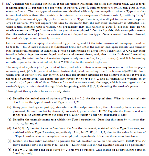
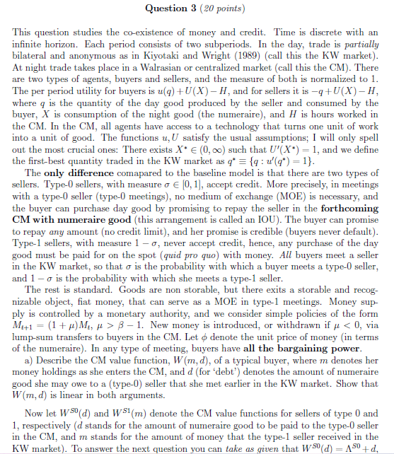
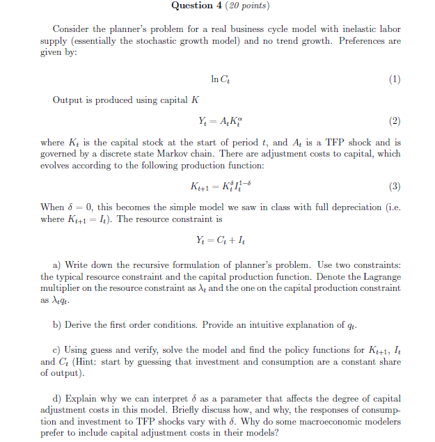
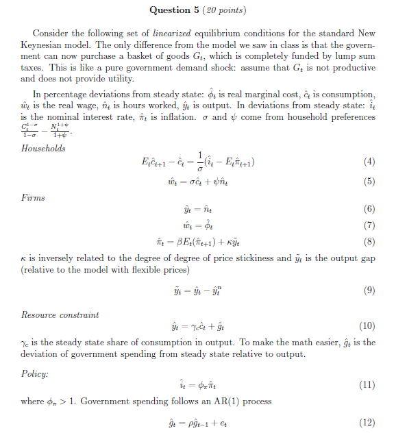
El. [2111} Consider the following extension ofthe MortensenPissarides model in continuous time. Labor force is normalized to l, but there are two types of workers, Type 1, with measure it E {I}, l}, and Type 2, with measure 1 ET. The two types of workers are identical with only one exception: when a Type i worker is matched with a rm, that match is terminated at an exogenous [Poisson] rate 35-, with A; 2:- 3.1.: Although rms would typically prefer to match with IType 1. workers, it is illegal to discriminate against Type 2 workers. \"5e will capture this idea by assuming that the matching technology is animal, i.e., when a rm matches with a worker, the probability that this worker is Type 1, depends only on the relative measure of Type 1 workers in the pool ofunemployed." On the ip side, this assumption means that the arrival rate of jobs to a worker does not depend on her type. Once a match has been formed, the worker's type is immediately revealed. Let the measure of unemployed workers of Type i be In, and let the total measure of unemployed workers be u = 111+ 113. A large measure of {identical} rms can enter the market and open exactly one vacancy [the equilibrium measure of vacancies, 13, will be determined by a free entry condition]. A C115 matching function brings together unemployed workers and vacant rms, and, due to the \"'I:I.I:Lbiased"I matching technology, the total number of matches depends only on 1.? and 1t, i.e., m. 2 tabs, 13], and it is increasing in both arguments. 21s is standard, let 5 E 13,311. denote the market tightness. The output ofa job is p Z:- {I per unit oftime, and while a rm is searching for a worker it has to pay a recruiting cost, 11!: 1':- D, per unit of time. Notice that, while searching, the rm has an expectation about which type of worker it will match with, and this expectation depends on the relative measure of types in the pool of unemployed .F'Lll agents discount future at the rate 1" 1':- , and all unemployed workers enjoy a benet 2 1':- per unit of time. t-Vhen a rm and a worker meet, the wage, which is contingent on the worker's type, is determined through Nash bargaining, with _S E {0,1} denoting the worker's power. Throughout this question focus on steady states. [all Describe the arrival rate of workers of Type E, t = l, 2, for the typical rnn. t-Vhat is the arrival rate o'fa rn: to the typical worker onype i, i: 1, 2'! {b} Using your ndings in part {a}, describe the Bevesidge curve {i.e., the relationship between unem ployment, LI", and market tightness, a} for each type of worker. EEIII: Equate the ows in and out of the pool ofunemployment for each type. Don't forget to use the exogenous 1T here. [ell Describe the unemployment rate within the Type i population. Denoting this term by '"r',-, show that \"TI '5: T3, To! any E. {d} Let V, J1,J3 denote the value functions ofa rm that is vacant, matched with a Type 1 worker, and matched with a Type 2 worker, respectively. Mso, let Hi, \"If, t = l, 2, denote the 1value functions of a Type t worker who is unemployed or employed, respectively. Describe these value functions. [ell Exploit the free entry condition to provide the job creation curve for this economy. I'Iint: The JG curve should relate the terms E, \"El, and my. Everything else in that equation should be a parameter. it} For t = l, 2, describe the wage curve {W'CI-J for type 1 workers. This should be a relationship between E and 1H,- {only}. Question 3 {21] points] This question studies the ooexistence of money and credit. Time is discrete with an innite horizon. Each period consists of two subperiods. In the day, trade is partially bilateral and anonymous as in Kiyotaki and Wright {1939] [call this the KW market]. At night trade takes place in a Walrasian or centralized market {call this the CM]. There are two types of agents, buyers and sellers, and the measure of both is normalized to l. The per period utility for buyers is u{q] + U{X] H, and for sellers it is g + UIIX} H, where q is the quantity of the day good produced by the seller and consumed by the buyer, X is consumption of the night good {the numeraire], and H is hours worked in the UM. In the CM, all agents have access to a technology that turns one unit of work into a unit of good. The Functions u,U satisfy the usual assumptions, I will only spell out the most crucial ones: There exists X' E {I}, on] such that U'{X"] = l, and we dene the rstbest quantity traded in the KW market as q' E {q : u'{q'] = I}. The only difference comapared to the baseline model is that there are two types of sellers. Type-[l sellers, with measure or IE [13,1], accept credit. More precisely, in meetings with a type-lll seller {type-[l meetings}, no medium of exchange {MOE} is necessary, and the buyer can purchase day good by promising to repay the seller in the forthcoming Chi with numeraire good {this arrangement is called an ICU]. The buyer can promise to repay any amount [no credit limit], and her promise is credible {buyers never default]. Type-l sellers, with measure 1 or, never accept credit, hence, any purchase of the day good must be paid for on the spot {quid pro quo] with money. All buyers meet a seller in the KW market, so that o" is the probability with which a buyer meets a type-[l seller, and l clr is the probability with which she meets a type-l seller. The rest is standard. Goods are non storable, but there exits a storable and recog nisable object, at money, that can serve as a MUE- in type-l meetings. Money sup ply is controlled by a monetary authority, and we consider simple policies of the form M,\" = {1 + p}M, p. 3.5 ,3 1. New money is introduced, or withdrawn if p. -=:: I], via lump-sum transfers to buyers in the CM. Let denote the unit price of money {in terms of the numeraire]. In any type of meeting, buyers have all the bargaining power. a} Describe the GM value function, WEm, d], of a typical buyer, where m denotes: her money holdings as she enters the CM, and d {for 'debt'] denotes the amount of numeraire good she may owe to a [typeD] seller that she met earlier in the KW market. Show that W{m, d] is linear in both arguments. Now let Wm{d] and W51{m] denote the CM value Functions for sellers of type I] and 1, respectively {at stands for the amount of numeraire good to be paid to the type[l seller in the CM, and m. stands for the amount of money that the type-l seller received in the KW market]. To answer the next question you can take as given that WEBM] = its\" + d, Question 4 {2E points} ISornsider the planner's problem for a real business cycle model with inelastic lab-or supply [essentially the stochastic growth model] and no trend growth. Preferences are given by: In Cr"; [1} Output is produced using capital H Y: = Riff? [2} where K; is the capital stock at the start of period t, and A; is a TFP shock and is governed by a discrete state Markov chain. There are adjustment costs to capital, which evolves according to the following production Function: Km = ll'5 [31' \"rhen 5 = D, this becomes the simple model we saw in class 1III.Iith full depreciation [i.e. where Kt\" = It}. The resource constraint is H=C+Ir a} Write down the recursive fonnulation of planner's problem. Use two constraints: the typical resource constraint and the capital production function. Denote the Lagrange multiplier on the resource constraint as Jo and the one on the capital production constraint as hm. b] Derive the rst order conditions. Provide an intuitive explanation of gg. c} Using guess and verify1 solve the model and nd the policy functions for KM], I, and Cr (Hint: start by guessing that investment and consumption are a constant share of output}. d] Explain whyr we can interpret 5 as a parameter that affects the degree of capital adjustment costs in this model. Briey discuss how1 and why, the responses of consump- tion and investment to TFP shocks vary with 5. Why do some macroeconomic modelers prefer to include capital adjustment costs in their models? Question 5 {EH points} Consider the following set of linearized equilibrium conditions for the standard New Keynesian model. The onlg,r di'erenoe from the model we saw in class is that the govern ment can now purchase a basket of goods Ch which is completely funded by lump sum taxes. This is like a pure government demand shock: assume that St is not productive and does not provide utility. In percentage deviations from steady state: oh is real marginal cost, E: is consumption1 11% is the real wage in is hours worked, y; is output. In deviations from stead}:r state: if is the nominal interest rate1 ii} is ination. o" and quit oome From household pneferenms El: _ El: 1: 1-115 ' Households 1 h Ere!\" C: = Eli: Eer+1l [4} air; = so; + on; [5} Firms 3}: = t [5} 13': = fl}: [7} 'Fl'i = .SEe'l''HIl + Ni: [8} we is inverselyr related to the degree of degree of price stickiness and , is the output gap {relative to the model with exible prices] is = 33 a}? [9} Resource constraint if: = \"has + rs {1D} qr: is the stead}.r state share of consumption in output. To make the math easier, t is the deviation of government spending from stead}.r state relative to output. Policy: . 1': = this {11} where t, 3.: 1. Government spending follows an ARIIZI} process : = P'bi + El: {12} For the rest of this question note that this model can be simplied to the familiar 3 equations: ass: s = ti as\" a") :13} fr; = ,SEr'l''HIl + m: {1'1} 3?: = $5er {15} Plus the process for government spending Eli = PER1 + 31!: \"El and a denition of the natural real rate of interest 0' F? = E1 - 1"]{1- :3le {17'} it: b] Using the method of undetermined oo-elcients1 nd the response of the output gap and ination to an exogenous increase in r; when prices are sticky and monetary policy follows the Taylor Rule above. To do this, guess that the solution for each variable is a linear function of the shock n: 1?: = hy! if: = Jig-e (Hint: follow the steps used in the problem set. Start by substituting the guesses, the monetary policy rule and the ARH} process for t into the dynamic equations [13} and {14).} c} How, and why, does the response of GDP differ from the model with exible prices? Do positive government spending shocks increase inflation? Provide economic intuition and {ifyou can] discuss the solution you found in part {b}. d] In principle, could monetary policy fully stabilize the output gap and ination after a govemment spending shock? (Hint: think about how the 3equation setup above looks like the cases we studied in class}? Would there be any additional benet from conducting optimal monetary policy under commitment
