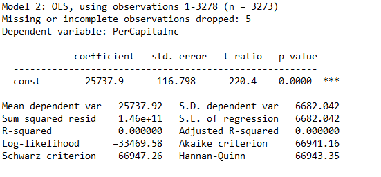
Model 2: OLS, using observations 1-3278 (n = 3273) Missing or incomplete observations dropped: 5 Dependent variable: PerCapitaInc coefficient std. error t-ratio p-value const 25737.9 116.798 220.4 0.0000 Mean dependent var 25737.92 S.D. dependent var 6682. 042 Sum squared resid 1. 46e+11 S. E. of regression 6682. 042 R-squared 0. 000000 Adjusted R-squared 0. 000000 Log-likelihood -33469.58 Akaike criterion 66941.16 Schwarz criterion 66947 . 26 Hannan-Quinn 66943.35(a) [1 point] Run a regression of per capita income (PerCapitaInc) on percent employment in the FIRE sector (PctEmpFIRE). What is the estimated slope? Explain what this number means in words in terms of per capita income and also indicate if the relationship is statistically significant at the 10%, 5%, and 1% levels. (b) [1 point] Run a regression of per capita income on percentage FIRE share, but now also include additional regressors: unemployment rate in 2010 (UnempRate2010) and percentage non-Hispanic white in 2010 (WhiteNon HispanicPct2010). Now, what is the estimated effect of percentage FIRE share on per capita income and also indicate if the relationship is statistically significant at the 10%, 5%, and 1% levels? (c) [2 points] Provide economic/econometric intuition as to why the effect of FIRE share on per capita income changed between parts (a) and (b). Note that I am asking you to think about the context (and hence the "story" behind these data). (d) [2 point] Construct a 95% confidence interval for the slope coefficient on PetEmpFIRE in (b). Write out your calculations. Clearly indicate how this confidence interval relates to whether PetEmpFIRE is statistically significant or not in this context.Model 3: OLS, using observations 1-3278 (n = 3271) Missing or incomplete observations dropped: 7 Dependent variable: PerCapitaInc coefficient std. error t-ratio p-value const 29979.7 556.990 53.82 0.0000 UnempRate2010 -845 . 858 30.7409 -27.52 4.32e-150 WhiteNonHispanic~ 50.6536 4. 69292 10.79 1. 04e-026 Mean dependent var 25730.05 5.D. dependent var 6673.982 Sum squared resid 1. 04e+11 S. E. of regression 5628.207 R-squared 0. 289271 Adjusted R-squared 0. 288836 F(2, 3268) 665.0465 P-value(F) 4.8e-243 Log-likelihood -32886.72 Akaike criterion 65779.44 Schwarz criterion 65797.72 Hannan-Quinn 65785.98