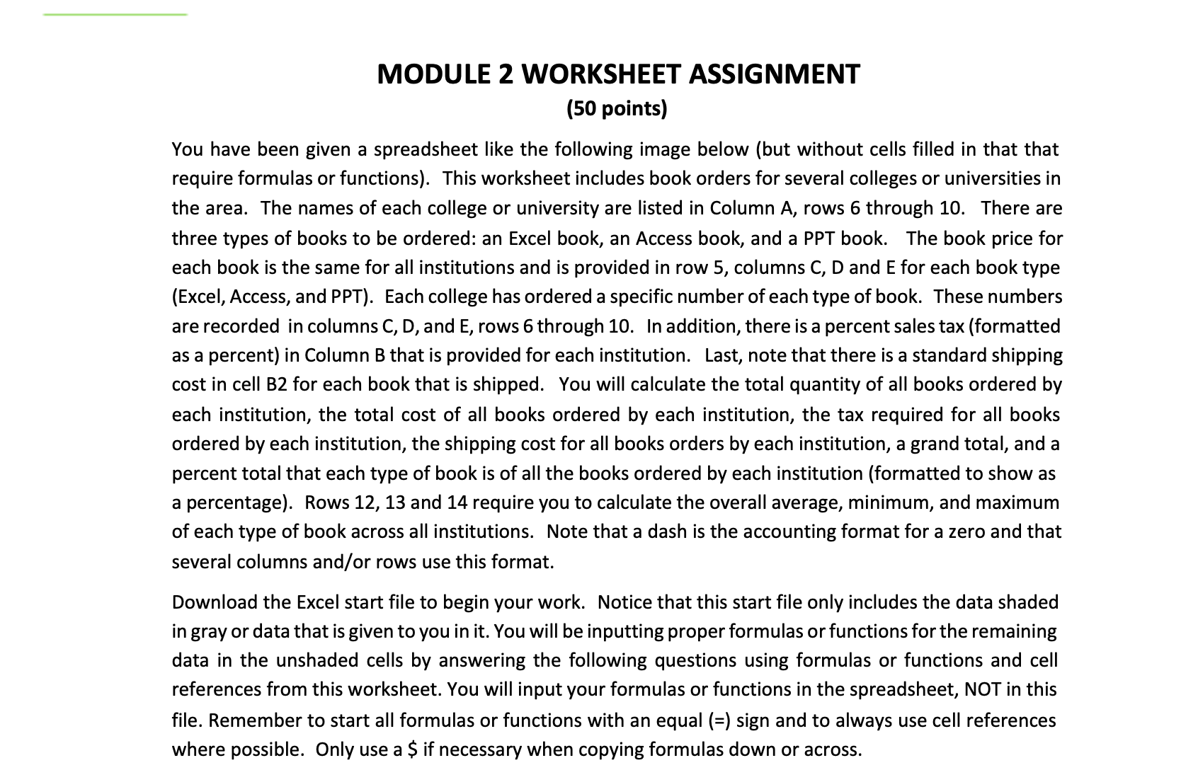
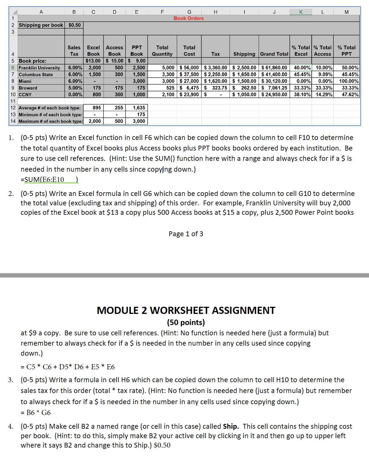
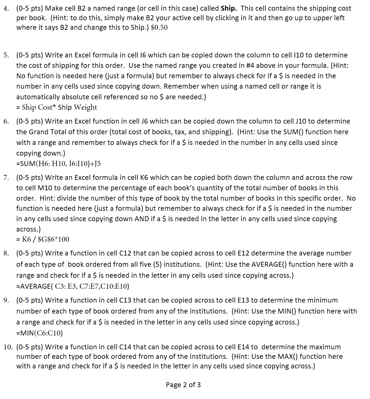
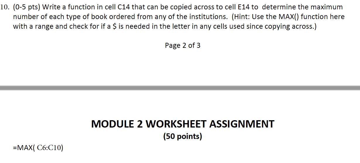
MODULE 2 WORKSHEET ASSIGNMENT (50 points) You have been given a spreadsheet like the following image below (but without cells filled in that that require formulas or functions). This worksheet includes book orders for several colleges or universities in the area. The names of each college or university are listed in Column A, rows 6 through 10. There are three types of books to be ordered: an Excel book, an Access book, and a PPT book. The book price for each book is the same for all institutions and is provided in row 5, columns C, D and E for each book type (Excel, Access, and PPT). Each college has ordered a specific number of each type of book. These numbers are recorded in columns C, D, and E, rows 6 through 10. In addition, there is a percent sales tax (formatted as a percent) in Column B that is provided for each institution. Last, note that there is a standard shipping cost in cell B2 for each book that is shipped. You will calculate the total quantity of all books ordered by each institution, the total cost of all books ordered by each institution, the tax required for all books ordered by each institution, the shipping cost for all books orders by each institution, a grand total, and a percent total that each type of book is of all the books ordered by each institution (formatted to show as a percentage). Rows 12, 13 and 14 require you to calculate the overall average, minimum, and maximum of each type of book across all institutions. Note that a dash is the accounting format for a zero and that several columns and/or rows use this format. Download the Excel start file to begin your work. Notice that this start file only includes the data shaded in gray or data that is given to you in it. You will be inputting proper formulas or functions for the remaining data in the unshaded cells by answering the following questions using formulas or functions and cell references from this worksheet. You will input your formulas or functions in the spreadsheet, NOT in this file. Remember to start all formulas or functions with an equal (=) sign and to always use cell references where possible. Only use a $ if necessary when copying formulas down or across. 723 A B 2 Shipping per book $0.50 0 D E F H J K L M Book Orders Sales 4 Tax 5 Book price: Excel Access PPT Book Book Book $13.00 $ 15.00 $ 9.00 Total Quantity Total Cost % Total % Total % Total Tax Shipping Grand Total Excel Access PPT 6 Franklin University 6.00% 2,000 500 2,500 7 Columbus State 6.00% 1,500 300 1,500 8 Miami 6.00% - 3,000 9 Broward 5.00% 175 175 175 10 CCNY 0.00% 800 300 1,000 5,000 $56,000 $3,360.00 $ 2,500.00 $ 61,860.00 3,300 $37,500 $2,250.00 $1,650.00 $ 41,400.00 3,000 $27,000 $1,620.00 $1,500.00 $30,120.00 525 $ 6,475 $ 323.75 $ 262.50 $ 7,061.25 2,100 $23,900 $ $1,050.00 $24,950.00 40.00% 10.00% 45.45% 9.09% 50.00% 0.00% 0.00% 33.33% 33.33% 38.10% 14.29% 45.45% 100.00% 33.33% 47.62% 11 12 Average # of each book type: 895 255 1,635 13 Minimum # of each book type: 175 14 Maximum # of each book type: 2,000 500 3,000 1. (0-5 pts) Write an Excel function in cell F6 which can be copied down the column to cell F10 to determine the total quantity of Excel books plus Access books plus PPT books books ordered by each institution. Be sure to use cell references. (Hint: Use the SUM() function here with a range and always check for if a $ is needed in the number in any cells since copying down.) =SUM(E6:E10 2. (0-5 pts) Write an Excel formula in cell G6 which can be copied down the column to cell G10 to determine the total value (excluding tax and shipping) of this order. For example, Franklin University will buy 2,000 copies of the Excel book at $13 a copy plus 500 Access books at $15 a copy, plus 2,500 Power Point books Page 1 of 3 MODULE 2 WORKSHEET ASSIGNMENT (50 points) at $9 a copy. Be sure to use cell references. (Hint: No function is needed here (just a formula) but remember to always check for if a $ is needed in the number in any cells used since copying down.) = C5 C6 + D5* D6 + E5 * E6 3. (0-5 pts) Write a formula in cell H6 which can be copied down the column to cell H10 to determine the sales tax for this order (total * tax rate). (Hint: No function is needed here (just a formula) but remember to always check for if a $ is needed in the number in any cells used since copying down.) = B6 * G6 4. (0-5 pts) Make cell B2 a named range (or cell in this case) called Ship. This cell contains the shipping cost per book. (Hint: to do this, simply make B2 your active cell by clicking in it and then go up to upper left where it says B2 and change this to Ship.) $0.50 4. (0-5 pts) Make cell B2 a named range (or cell in this case) called Ship. This cell contains the shipping cost per book. (Hint: to do this, simply make B2 your active cell by clicking in it and then go up to upper left where it says B2 and change this to Ship.) $0.50 5. (0-5 pts) Write an Excel formula in cell 16 which can be copied down the column to cell I10 to determine the cost of shipping for this order. Use the named range you created in #4 above in your formula. (Hint: No function is needed here (just a formula) but remember to always check for if a $ is needed in the number in any cells used since copying down. Remember when using a named cell or range it is automatically absolute cell referenced so no $ are needed.) = Ship Cost* Ship Weight 6. (0-5 pts) Write an Excel function in cell J6 which can be copied down the column to cell J10 to determine the Grand Total of this order (total cost of books, tax, and shipping). (Hint: Use the SUM() function here with a range and remember to always check for if a $ is needed in the number in any cells used since copying down.) =SUM(H6: H10, 16:110)+J5 7. (0-5 pts) Write an Excel formula in cell K6 which can be copied both down the column and across the row to cell M10 to determine the percentage of each book's quantity of the total number of books in this order. Hint: divide the number of this type of book by the total number of books in this specific order. No function is needed here (just a formula) but remember to always check for if a $ is needed in the number in any cells used since copying down AND if a $ is needed in the letter in any cells used since copying across.) = K6 / $G$6*100 8. (0-5 pts) Write a function in cell C12 that can be copied across to cell E12 determine the average number of each type of book ordered from all five (5) institutions. (Hint: Use the AVERAGE() function here with a range and check for if a $ is needed in the letter in any cells used since copying across.) =AVERAGE( C3: E3, C7:E7,C10:E10) 9. (0-5 pts) Write a function in cell C13 that can be copied across to cell E13 to determine the minimum number of each type of book ordered from any of the institutions. (Hint: Use the MIN() function here with a range and check for if a $ is needed in the letter in any cells used since copying across.) =MIN(C6:C10) 10. (0-5 pts) Write a function in cell C14 that can be copied across to cell E14 to determine the maximum number of each type of book ordered from any of the institutions. (Hint: Use the MAX() function here with a range and check for if a $ is needed in the letter in any cells used since copying across.) Page 2 of 3 10. (0-5 pts) Write a function in cell C14 that can be copied across to cell E14 to determine the maximum number of each type of book ordered from any of the institutions. (Hint: Use the MAX() function here with a range and check for if a $ is needed in the letter in any cells used since copying across.) =MAX(C6:C10) Page 2 of 3 MODULE 2 WORKSHEET ASSIGNMENT (50 points)