need help:-
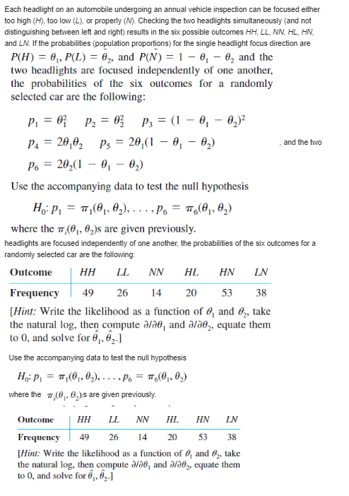
Each headlight on an automobile undergoing an annual vehicle inspection can be focused either too high (H), too low (L), or properly (N). Checking the two headlights simultaneously (and not distinguishing between left and right) results in the six possible outcomes HH, LL, NN, HL, HN, and L/. If the probabilities (population proportions) for the single headlight focus direction are P(H) = 01, P(L) = 62, and P(N) = 1 - 0, - 6, and the two headlights are focused independently of one another, the probabilities of the six outcomes for a randomly selected car are the following: P1 = 0; P2 = 02 P3 = (1 -01 - 02)2 PA = 20, 02 Ps = 20, (1 - 0, - #2) and the two Po = 202(1 - 0, - 02) Use the accompanying data to test the null hypothesis Hop, = TT, (0, , 02 ), . . . . Po = To (0,, 02) where the w,(0,, 0,)s are given previously. headlights are focused independently of one another, the probabilities of the six outcomes for a randomly selected car are the following: Outcome HH LL NN HL HN LN Frequency 49 26 14 20 53 38 [Hint: Write the likelihood as a function of 6, and &, take the natural log, then compute a/ad, and a/ad,, equate them to 0, and solve for #1, 02.] Use the accompanying data to test the null hypothesis Hop = #, (0,,02). . . .. P6 = T 6(0,, 02) where the + (0 , 0, )is are given previously. Outcome HH LL NN HL HN IN Frequency 49 26 14 20 53 38 [Hint: Write the likelihood as a function of 6, and 62, take the natural log, then compute a/20, and a/362, equate them to 0, and solve for . #2.]If a process variable is normally distributed, in the long run virtually all observed values should be between u - 30 and u + 30 , giving a process spread of 60. a. With LSL and USL denoting the lower and upper specification limits, one commonly used process capability index is u - 30 . The value Co = 1 indicates a process that is only marginally capable of meeting specifications. Ideally, C. should exceed 1.33 (a "very good" process). Calculate the value of C, for each of the cork production processes described in the previous exercise, and comment. b. The Co index described in (a) does not take into account process location. A capability measure that does involve the process mean is M + 30. Calculate the value of Cox for each of the cork-production processes described in the previous exercise, and comment. [Vote: In practice, m and s have to be estimated from process data; we show how to do this in Section 16.2] c. How do Go and Gok compare, and when are they equal?In the case of known u and o, what control limits are necessary for the probability of a single point being outside the limits for an in-control process to be .005?Calculate control limits for an $ chart from the refractive index data of Exercise 11. Does the process appear to be in control with respect to variability? Why or why not? Reference exercise 11 The accompanying table gives sample means and standard deviations, each based on n = 6 observations of the refractive index of fiber-optic cable. Construct a control chart, and comment on its appearance. [Mine, Ex, = 2317.07 and Ss; = 30.34.]and Day Day 95.47 1.30 13 97.02 1.28 97.38 88 14 95.55 1.14 96.85 1.43 15 96.29 1.37 NOUAWNE 96.64 1.59 16 96.80 1.40 96.87 1.52 17 96.01 1.58 96.52 1.27 18 95.39 .98 96.08 1.16 19 96.58 1.21 96.48 .79 20 96.43 .75 96.63 1.48 21 97.06 1.34 10 96.50 .80 22 98.34 1.60 11 97.22 1.42 23 96.42 1.22 12 96.55 1.65 24 95.99 1.18 Day Day 95.47 1.30 13 97.02 1.28 97.38 .88 14 95.55 1.14 96.85 1.43 15 96.29 1.37 96.64 1.59 16 96.80 1.40 96.87 1.52 17 96.01 1.58 96.52 1.27 18 95.39 98 96.08 1.16 19 96.58 1.21 96.48 .79 20 96.43 .75 96.63 1.48 21 97.06 1.34 10 96.50 .80 22 98.34 1.60 11 97.22 1.42 23 96.42 1.22 12 96.55 1.65 24 95.99 1.18When S" is the sample variance of a normal random sample, $ has a chi-squared distribution with n - 1 di, so (# - 1)572 This suggests that an alternative chart for controlling process variation involves plotting the sample variances and using the control limits XML = 998 from which Xmeg Xmal =.998 A - I 1 - 1 Construct the corresponding chart for the data of Exercise 11. [Hint: The lower- and upper-tailed chi-squared critical values for 5 of are .210 and 20.515, respectively.] Reference exercise 11 The accompanying table gives sample means and standard deviations, each based on n = 6 observations of the refractive index of fiber-optic cable. Construct a control chart, and comment on its appearance. [Hint: Ex, = 2317.07 and Es, = 30.34.]and Day Day 95.47 1.30 13 97.02 1.28 97.38 88 14 WN 95.55 1.14 96.85 1.43 15 96.29 1.37 96.64 1.59 16 96.80 1.40 96.87 1.52 17 96.01 1.58 96.52 1.27 18 95.39 98 96.08 1.16 19 96.58 1.21 96.48 .79 20 96.43 .75 96.63 1.48 21 97.06 1.34 10 96.50 .80 22 98.34 1.60 11 97.22 1.42 23 96.42 1.22 12 96.55 1.65 24 95.99 1.18 Day Day 95.47 1.30 13 97.02 1.28 97.38 88 14 95.55 1.14 96.85 1.43 15 96.29 1.37 GUAWN- 96.64 1.59 16 96.80 1.40 96.87 1.52 17 96.01 1.58 96.52 1.27 18 95.39 .98 96.08 1.16 19 96.58 1.21 96.48 .79 20 96.43 75 96.63 1.48 21 97.06 1.34 10 96.50 .80 22 98.34 1.60 11 97.22 1.42 23 96.42 1.22 12 96.55 1.65 24 95.99 1.18


