Need help on chapter 7 excel project on simnet

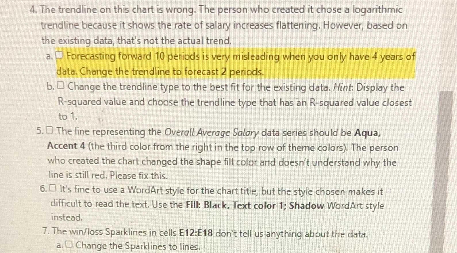
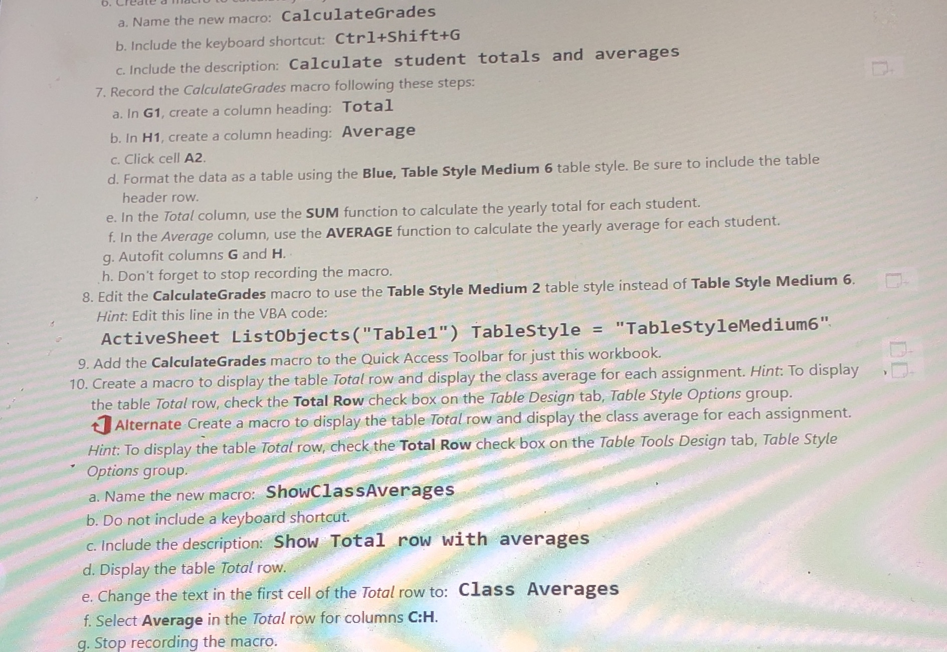
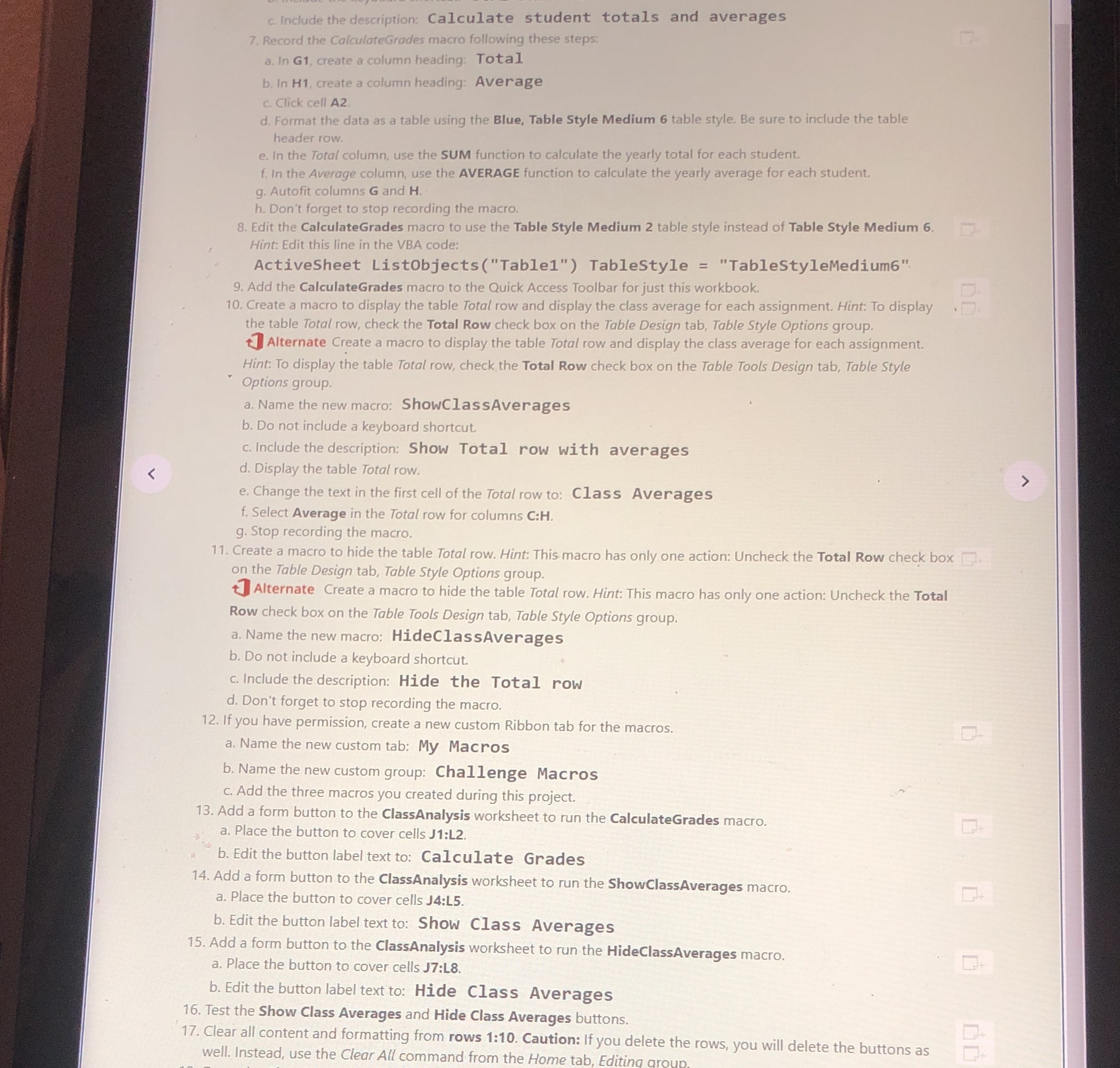
4. The trendline on this chart is wrong. The person who created it chose a logarithmic trendline because it shows the rate of salary increases flattening, However, based on the existing data, that's not the actual trend. a. Forecasting forward 10 periods is very misleading when you only have 4 years of data. Change the trendline to forecast 2 periods. b. Change the trendline type to the best fit for the existing data. Hint: Display the R-squared value and choose the trendline type that has an R-squared value closest to 1. 5. The line representing the Overall Average Salary data series should be Aqua, Accent 4 (the third color from the right in the top row of theme colors). The person who created the chart changed the shape fill color and doesn't understand why the line is still red. Please fix this. 6. It's fine to use a WordArt style for the chart title, but the style chosen makes it difficult to read the text. Use the Fill: Black, Text color 1; Shadow WordArt style instead. 7. The win/loss Sparklines in cells E12:E18 don't tell us anything about the data. a. Change the Sparklines to lines.a. Name the new macro: CalculateGrades b. Include the keyboard shortcut: Ctr1+Shift+G c. Include the description: Calculate student totals and averages 7. Record the CalculateGrades macro following these steps: a. In G1, create a column heading: Total b. In H1, create a column heading: Average c. Click cell A2. d. Format the data as a table using the Blue, Table Style Medium 6 table style. Be sure to include the table header row . e. In the Total column, use the SUM function to calculate the yearly total for each student. f. In the Average column, use the AVERAGE function to calculate the yearly average for each student. g. Autofit columns G and H. h. Don't forget to stop recording the macro. 8. Edit the CalculateGrades macro to use the Table Style Medium 2 table style instead of Table Style Medium 6. Hint: Edit this line in the VBA code: ActiveSheet ListObjects ("Table1") TableStyle = "TableStyleMedium6" 9. Add the CalculateGrades macro to the Quick Access Toolbar for just this workbook. 10. Create a macro to display the table Total row and display the class average for each assignment. Hint: To display the table Total row, check the Total Row check box on the Table Design tab, Table Style Options group. Alternate Create a macro to display the table Total row and display the class average for each assignment. Hint: To display the table Total row, check the Total Row check box on the Table Tools Design tab, Table Style Options group. a. Name the new macro: ShowClassAverages b. Do not include a keyboard shortcut. c. Include the description: Show Total row with averages d. Display the table Total row. e. Change the text in the first cell of the Total row to: Class Averages f. Select Average in the Total row for columns C:H. g. Stop recording the macro.c. Include the description: Calculate student totals and averages 7. Record the CalculateGrades macro following these steps: a. In G1, create a column heading: Total b. In H1, create a column heading: Average c. Click cell A2. d. Format the data as a table using the Blue, Table Style Medium 6 table style. Be sure to include the table header row. e. In the Total column, use the SUM function to calculate the yearly total for each student. f. In the Average column, use the AVERAGE function to calculate the yearly average for each student. g. Autofit columns G and H. h. Don't forget to stop recording the macro. 8. Edit the CalculateGrades macro to use the Table Style Medium 2 table style instead of Table Style Medium 6. Hint: Edit this line in the VBA code: ActiveSheet ListObjects("Table1") TableStyle = "TableStyleMedium6" 9. Add the CalculateGrades macro to the Quick Access Toolbar for just this workbook. 10. Create a macro to display the table Total row and display the class average for each assignment. Hint: To display the table Total row, check the Total Row check box on the Table Design tab, Table Style Options group. Alternate Create a macro to display the table Total row and display the class average for each assignment. Hint: To display the table Total row, check the Total Row check box on the Table Tools Design tab, Table Style Options group. a. Name the new macro: ShowClassAverages b. Do not include a keyboard shortcut. c. Include the description: Show Total row with averages d. Display the table Total row. e. Change the text in the first cell of the Total row to: Class Averages f. Select Average in the Total row for columns C:H. g. Stop recording the macro. 11. Create a macro to hide the table Total row. Hint: This macro has only one action: Uncheck the Total Row check box on the Table Design tab, Table Style Options group. Alternate Create a macro to hide the table Total row. Hint: This macro has only one action: Uncheck the Total Row check box on the Table Tools Design tab, Table Style Options group. a. Name the new macro: HideClassAverages b. Do not include a keyboard shortcut. c. Include the description: Hide the Total row d. Don't forget to stop recording the macro. 12. If you have permission, create a new custom Ribbon tab for the macros. a. Name the new custom tab: My Macros b. Name the new custom group: Challenge Macros c. Add the three macros you created during this project. 13. Add a form button to the ClassAnalysis worksheet to run the CalculateGrades macro. a. Place the button to cover cells J1:L2. "b. Edit the button label text to: Calculate Grades 14. Add a form button to the ClassAnalysis worksheet to run the ShowClassAverages macro. a. Place the button to cover cells J4:15. b. Edit the button label text to: Show Class Averages 15. Add a form button to the ClassAnalysis worksheet to run the HideClassAverages macro. a. Place the button to cover cells J7:L8. b. Edit the button label text to: Hide Class Averages 16. Test the Show Class Averages and Hide Class Averages buttons. 17. Clear all content and formatting from rows 1:10. Caution: If you delete the rows, you will delete the buttons as well. Instead, use the Clear All command from the Home tab, Editing