Need help starting this prep task.
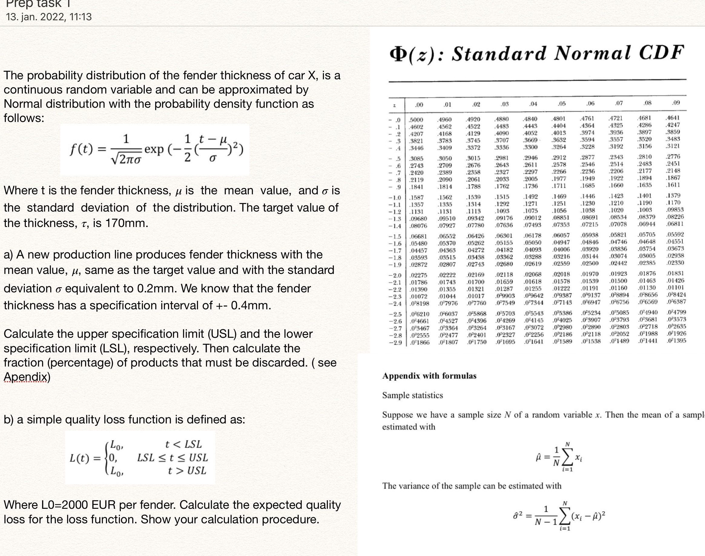
Prep task 13. jan. 2022, 11:13 P(z) : Standard Normal CDF The probability distribution of the fender thickness of car X, is a continuous random variable and can be approximated by Normal distribution with the probability density function as .00 .0 .02 .03 .04 .05 .06 .07 .08 09 follows: 4960 4920 4880 4840 4801 476 4721 4681 .4641 5000 4602 .4562 4522 4483 4443 .4404 .4364 4325 4286 .4247 .4207 .4168 4129 .4090 .4052 4013 .3974 .3936 .3897 .3859 3821 .3783 .3745 3707 3669 3632 .3594 3557 .3520 .3483 2 ) 9336 3264 .3228 3192 .3121 f (t) = .3409 3379 3300 V2no exp (- 2 3446 3156 .3050 3015 .2981 2946 .2877 2343 2810 .2776 .3085 2709 .2676 2643 2578 2546 2514 2483 2743 2611 .2451 .2358 .2327 2297 2266 2236 2206 2177 .2148 .2420 .2389 2119 2090 2061 2033 .2005 1977 .1949 1922 1894 1867 1814 1762 1685 1635 1841 .1788 1736 1711 1660 .1611 Where t is the fender thickness, u is the mean value, and o is 1379 - 1.0 .1587 .1562 1539 1515 1492 1469 .1446 1423 1401 -1.1 .1335 1314 1292 1271 1251 1230 .1210 .1 190 .1170 the standard deviation of the distribution. The target value of 1357 -1.2 .1131 .1131 .1113 1093 ,1075 .1050 .1038 . 1020 .1003 .09853 1.3 .09680 .09510 .09342 09176 09012 .08851 08691 08534 08379 .08226 the thickness, t, is 170mm. .07927 07780 .07493 07353 07215 .07078 .06944 0681 1 -1.4 08076 07636 -1.5 .06681 .06552 06426 .06301 06178 06057 .05938 .05821 .05705 .05592 -1.6 .05480 .05370 .05262 05155 05050 .04947 .04846 .04746 .04648 .04551 -1.7 .04363 .04272 .04182 .04093 04006 03920 03836 03754 .03673 .04457 a) A new production line produces fender thickness with the -18 .03593 03515 .02438 .03362 03988 03216 .03144 03074 .03005 .02938 -1.9 02872 .02807 02743 .02680 02619 02559 02500 02442 02385 02330 mean value, M, same as the target value and with the standard .01831 -2.0 .02275 .02222 .02169 .02118 .02068 02018 01970 .01923 .01876 -2.1 .01786 .01743 .01700 .01659 .01618 .01578 .01539 .01500 .01463 .01426 deviation o equivalent to 0.2mm. We know that the fender -2.2 .01390 01355 01321 .01287 .01255 .01222 .01191 .01160 .01130 .01 101 -2.3 .01072 .01044 .01017 .09903 .029642 .09387 .09137 .0 8894 .0-8656 .0 8424 thickness has a specification interval of +- 0.4mm. -2.4 .0 8198 027976 .0-7760 .0'7549 .0 7344 0-7143 .0 6947 .026756 .0 6569 .0 6387 -2.5 .0 6210 .0-6037 .0:5868 .0:5703 .025543 .0-5386 .0 5234 .0'5085 024940 .0'4799 -2.6 .0-4661 .0-4527 .0 4396 .0 4269 .0-4145 .0-4025 .0 3907 .023793 .023681 .0'3573 -2.7 .0 3467 .0 3364 .0 3264 .0:3167 .0-3072 0 2980 .0:2890 .0'2803 0-2718 .092635 Calculate the upper specification limit (USL) and the lower -2.8 .0 2555 .0:2477 .0:2401 .0 2327 .0-2256 .0 2186 .0-21 18 .0'2052 .0'1988 .0'1926 -2.9 .0 1866 .0=1807 .0'1750 .0 1695 .0 1641 .0 1589 .0-1538 .0'1489 .0*1441 .0'1395 specification limit (LSL), respectively. Then calculate the fraction (percentage) of products that must be discarded. ( see Apendix) Appendix with formulas Sample statistics Suppose we have a sample size N of a random variable x. Then the mean of a sampl b) a simple quality loss function is defined as: estimated with Lo' t USL The variance of the sample can be estimated with Where LO=2000 EUR per fender. Calculate the expected quality loss for the loss function. Show your calculation procedure. 82 1 5( x 1 - 1 ) 2 N - 12


