need help with graph as well

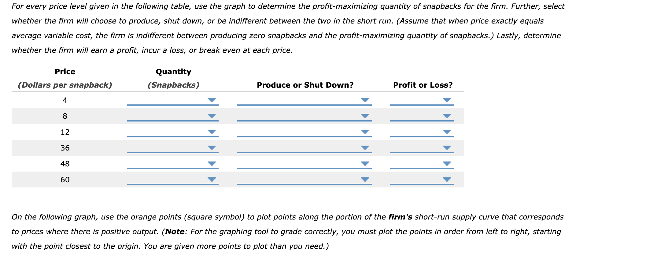
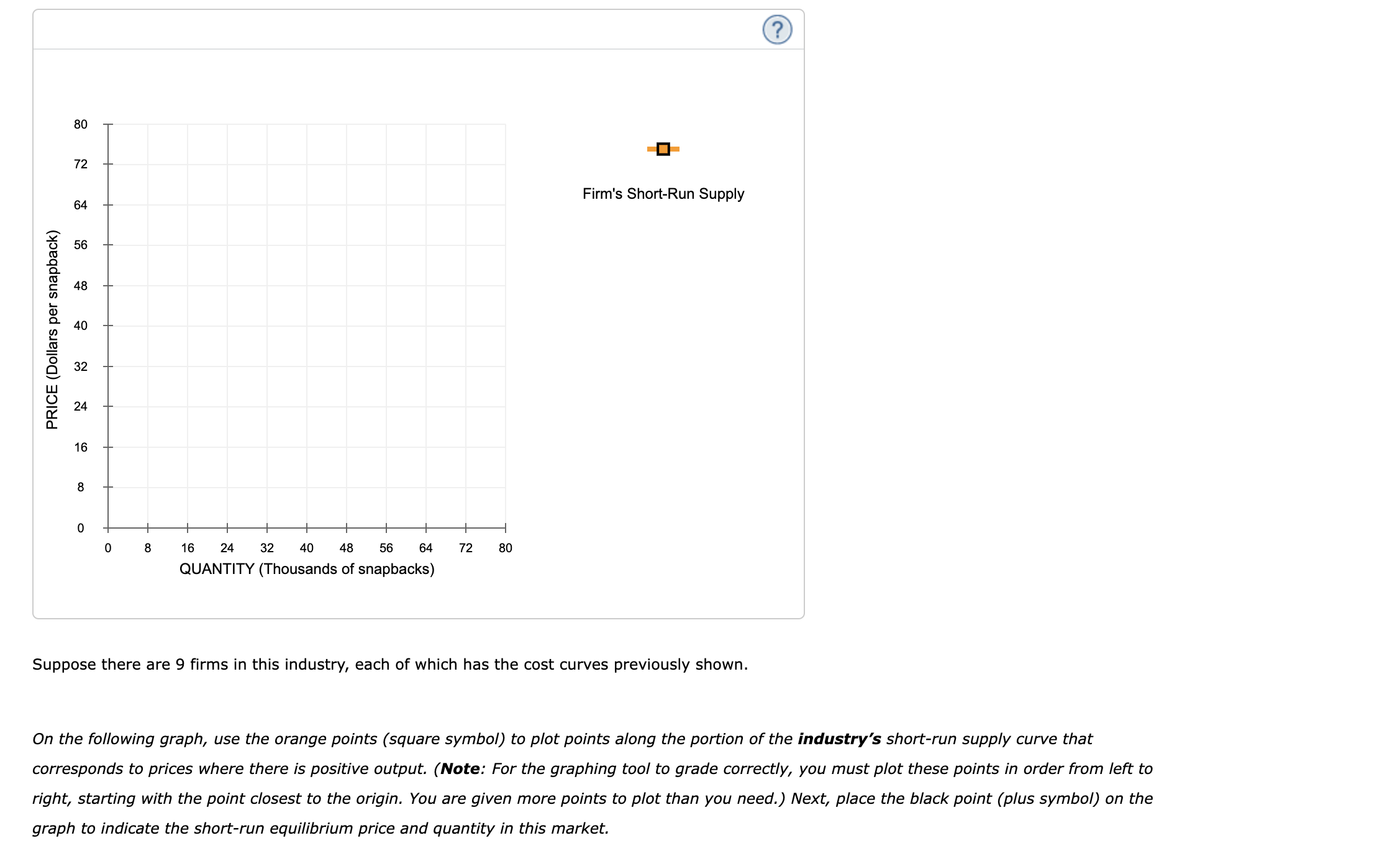
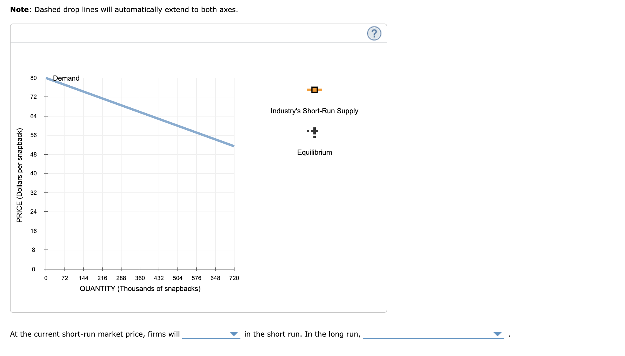
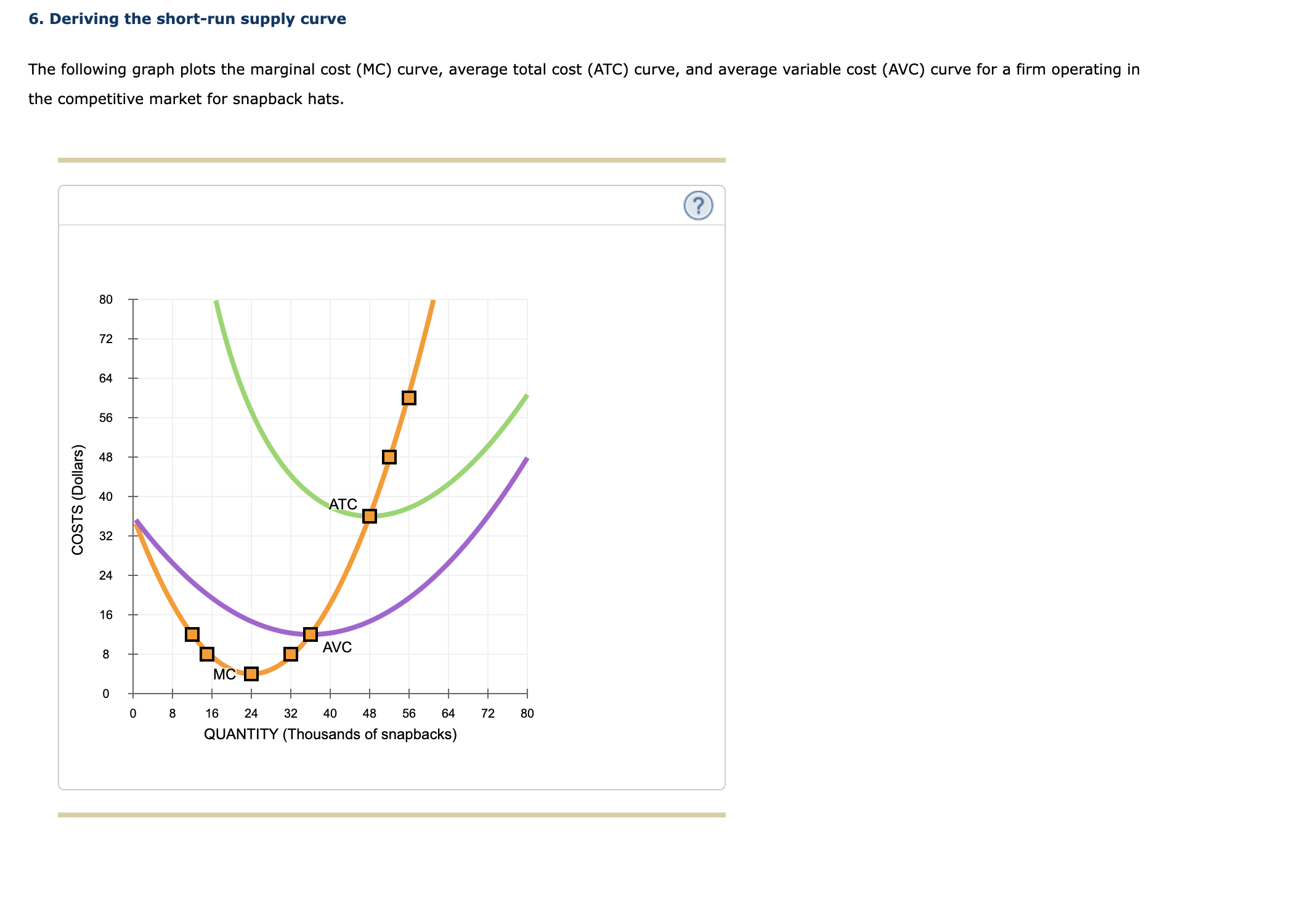
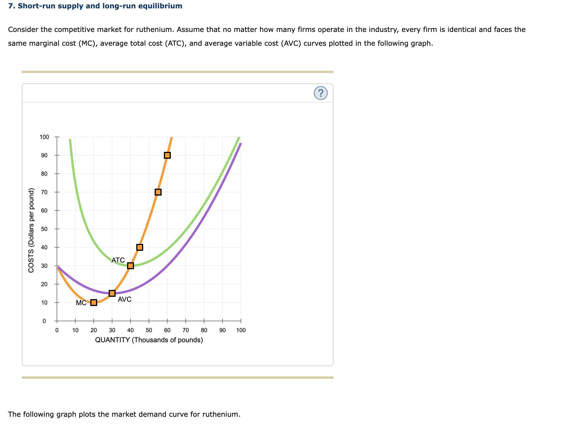
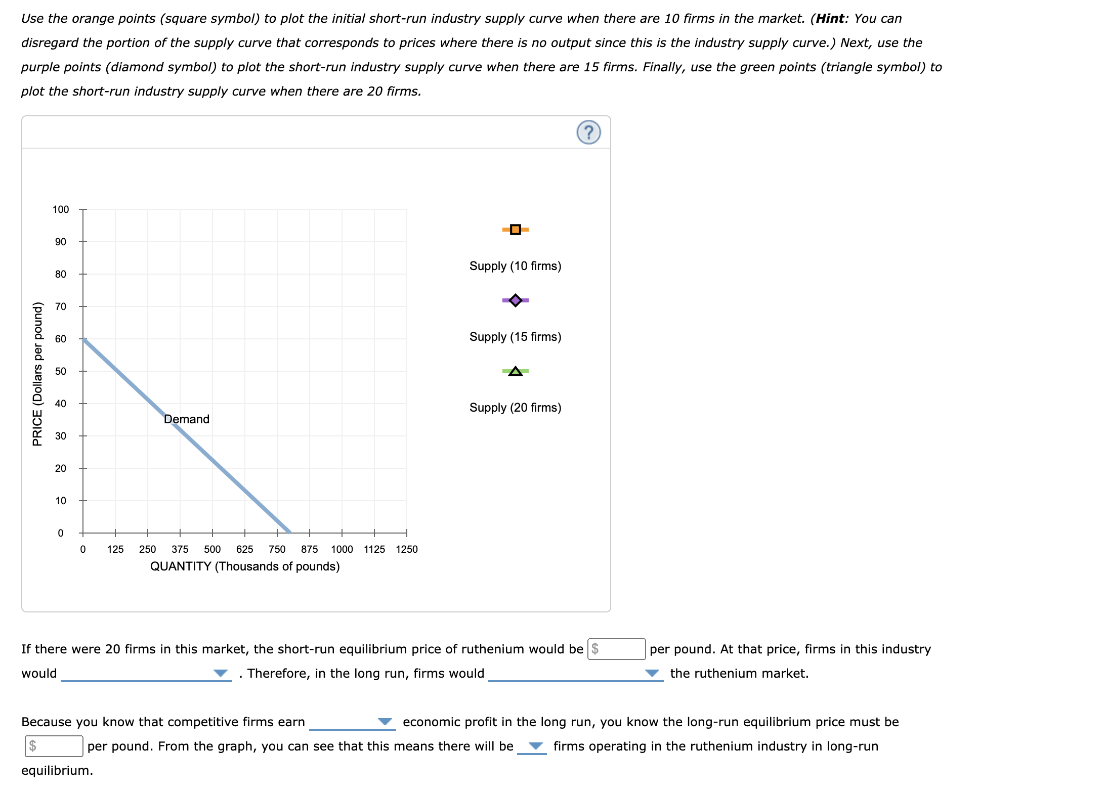
6. Deriving the short-run supply curve The following graph plots the marginal cost (MC) curve, average total cost (ATC) curve, and average variable cost (AVC) curve for a firm operating in the competitive market for snapback hats. (? 80 12 64 56 48 COSTS (Dollars) 40 ATC 32 24 16 AVC MC 8 16 24 32 40 48 56 64 72 80 QUANTITY (Thousands of snapbacks)For every price level given in the following table, use the graph to determine the prot-maximizing quantity of snapbacks for the rm. Further, select whether the rm will choose to produce, shut down, or be indifferent between the two in the short run. (Assume that when price exactly equals average variable cost, the rm is indifferent between producing zero snapbacks and the prot-maximizing quantity of snapbacks.) Lastly, determine whether the rm will earn a prot, incur a loss, or break even at each price. Price Quantity (Dollars per snapback) (Snapbacks) Produce or Shut Down? Profit or Loss? 4 v v v 8 V V v 12 Y Y Y 36 V v v 48 V V Y 60 v v v On the following graph, use the orange points (square symbol) to plot points along the portion of the rm '5 short-run supply curve that corresponds to prices where there is positive output. (Note: For the graphing tool to grade correctly, you must plot the points in order from left to right, starting with the point closest to the origin. You are given more points to plot than you need.) 30 El 72 64 Firm's Short-Run Supply 56 48 40 32 24 PRICE (Dollars per snapback) 16 0 l l l l l l l l l | O 8 16 24 32 40 4B 56 64 72 80 QUANTITY (Thousands of snapbacks) Suppose there are 9 firms in this industry, each of which has the cost curves previously shown. On the following graph, use the orange points (square symbol) to plot points along the portion of the industry's shortrun supply curve that corresponds to prices where there is positive output. (Note: For the graphing tool to grade correctly, you must plot these points in order from left to right, starting with the point closest to the origin. You are given more points to plot than you need.) Next, place the black point (plus symbol) on the graph to indicate the shortrun equilibrium price and quantity in this market. Note: Dashed drop lines will automatically extend to both axes. 80 Demand 72 Industry's Short-Run Supply 64 56 -+ 48 Equilibrium 40 PRICE (Dollars per snapback) 32 24 16 8 0 72 144 216 288 360 432 504 576 648 720 QUANTITY (Thousands of snapbacks) At the current short-run market price, firms will in the short run. In the long run,7. Short-run supply and long-run equilibrium Consider the competitive market for ruthenium. Assume that no matter how many firms operate in the industry, every firm is identical and faces the same marginal cost (MC), average total cost (ATC), and average variable cost (AVC) curves plotted in the following graph. (5?? 100 90 80 70 60 50 40 30 COSTS (Dollars per pound) 20 o 10 20 so 40 50 60 70 80 90 100 QUANTITY (Thousands of pounds) The following graph plots the market demand curve for ruthenium. Use the orange points (square symbol) to plot the initial shortrun industry supply curve when there are 10 rms in the market. (Hint: You can disregard the portion of the supply curve that corresponds to prices where there is no output since this is the industry supply curve.) Next, use the purple points (diamond symbol) to plot the shortrun industry supply curve when there are 15 rms. Finally, use the green points (triangle symbol) to plot the shortrun industry supply curve when there are 20 rms. 100 El 90 -- 60 __ Supply (10 rms) 3 7o + o. 60 _. Supply (15rms) E m E 50 - A E 40 s | (20f ) V _ uppy Irms If: Demand E 30 - 20 - 1o 0 l l l l l l l l l l 0 125 250 375 500 625 750 875 1000 1125 1250 QUANTITY (Thousands of pounds) If there were 20 firms in this market, the shortrun equilibrium price of ruthenium would be C] per pound. At that price, firms in this industry would V . Therefore, in the long run, firms would V the ruthenium market. Because you know that competitive firms earn V economic profit in the long run, you know the long-run equilibrium price must be C] per pound. From the graph, you can see that this means there will be V firms operating in the ruthenium industry in longrun equilibrium. True or False: Assuming implicit costs are positive, each of the firms operating in this industry in the long run earns positive accounting profit. 0 True 0 False