Need help with parts b,c, and d please
need help figuring out how to do the sensitivity analysis please provide me with the steps/formulas
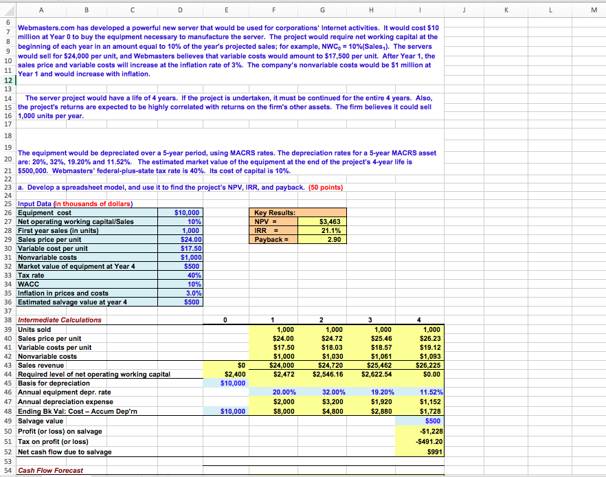
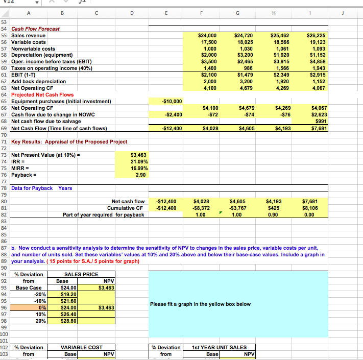
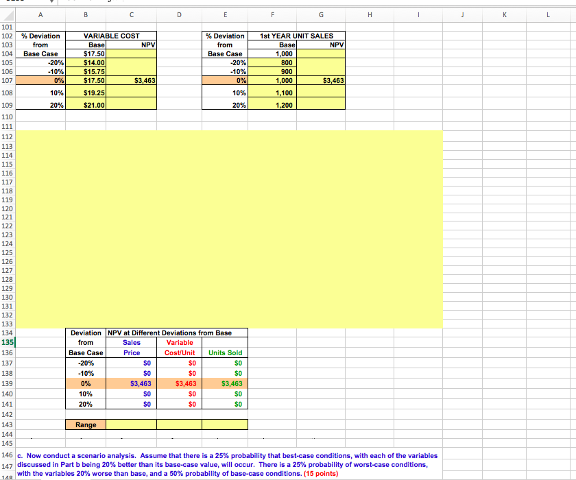
C D E F J K L M Webmasters.com has developed a powerful new server that would be used for corporations' Internet activities. It would cost $10 million at Year O to buy the equipment necessary to manufacture the server. The project would require net working capital at the beginning of each year in an amount equal to 10% of the year's projected sales; for example, NWC = 10%(Sales). The servers would sell for $24,000 per unit, and Webmasters believes that variable costs would amount to $17,500 per unit. After Year 1, the sales price and variable costs will increase at the inflation rate of 3%. The company's nonvariable costs would be $1 million at Year 1 and would increase with inflation. The server project would have a life of 4 years. If the project is undertaken, it must be continued for the entire 4 years. Also, 15 the project's returns are expected to be highly correlated with returns on the firm's other assets. The firm believes it could sell 16 1,000 units per year. 17 The equipment would be depreciated over a 5-year period, using MACRS rates. The depreciation rates for a 5-year MACRS asset are: 20%, 32%, 19.20% and 11.52%. The estimated market value of the equipment at the end of the project's 4-year life is $500,000. Webmasters' federal-plus-state tax rate is 40%. Its cost of capital is 10%. 23 a. Develop a spreadsheet model, and use it to find the project's NPV, IRR, and payback. (50 points) 24 25 Input Data fin thousands of dollars) 26 Equipment cost $10.000 Key Results: 27 Net operating working capital/Sales I 10% NPV = $3.463 28 First year sales (in units) 1.000 IRR = 21.1% 29 Sales price per unit $24.00 Payback = 2.90 30 Variable cost per unit $17.50 31 Nonvariable costs $1,000 32 Market value of equipment at Year 4 S500 33 Tax rate 40% 34 WACC 10% 35 Inflation in prices and costs 3.0% 36 Estimated salvage value at year 4 $500 1,000 $24.00 $17.50 $1,000 $24,000 $2,472 1,000 $24.72 $18.03 $1,030 $24,720 $2,546.16 1,000 $25.46 $18.57 $1,061 $25,462 $2,622.54 1,000 $26.23 $19.12 $1,093 $26,225 $0.00 38 Intermediate Calculations 39 Units sold 40 Sales price per unit 41 Variable costs per unit 42 Nonvariable costs 43 Sales revenue 44 Required level of net operating working capital 45 Basis for depreciation 46 Annual equipment depr. rate 47 Annual depreciation expense 48 Ending Bk Val: Cost - Accum Depirn 49 Salvage value 50 Profit (or loss) on salvage 51 Tax on profit (or loss) 52 Net cash flow due to salvage $2,400 $10,000 20.00% $2,000 $8,000 32.00% $3,200 $4,800 19.20% $1,920 $2,880 $10,000 11.52% $1,152 $1,728 $500 -$1,228 -$491.20 $991 54 Cash Flow Forecast H 53 54 Cash Flow Forecast 55 Sales revenue 56 Variable costs 57 Nonvariable costs 58 Depreciation (equipment) 59 Oper. income before taxes (EBIT) 60 Taxes on operating income (40%) 61 EBIT (1-1) 62 Add back depreciation 63 Net Operating CF 64 Projected Net Cash Flows 65 Equipment purchases (Initial Investment) 66 Net Operating CF 67 Cash flow due to change in NOWC 68 Net cash flow due to salvage 69 Net Cash Flow (Time line of cash flows) 70 71 Key Results: Appraisal of the Proposed Project $24,000 17,500 1.000 $2,000 $3,500 1,400 $2,100 2,000 4,100 $24,720 18,025 1.030 $3,200 $2,465 986 $1,479 3,200 4,679 $25,462 18,566 1,061 $1,920 $3,915 1,566 $2,349 1,920 4,269 $26,225 19,123 1.093 $1,152 $4,858 1,943 $2,915 1,152 4,067 -$10,000 $4,100 -$72 $4,679 -$74 $4,269 -$76 -$2,400 $4,067 $2,623 $991 $7,681 -$12,400 $4,028 $4,605 $4,193 73 Net Present Value (at 10%) = 74 IRR = 75 MIRR = 76 Payback = $3,463 21.09% 16.99% 2.90 77 78 Data for Payback Years 79 80 Net cash flow Cumulative CF Part of year required for payback -$12,400 -$12,400 81 $4,028 -$8,372 1.00 $4,605 -$3,767 1.00 $4,193 $425 0.90 $7,681 $8,106 0.00 83 85 86 87 b. Now conduct a sensitivity analysis to determine the sensitivity of NPV to changes in the sales price, variable costs per unit, 88 and number of units sold. Set these variables' values at 10% and 20% above and below their base-case values. Include a graph in 89 your analysis. (15 points for S.A.J 5 points for graph) 90 91 92 Base 94 % Deviation from Base Case -20% -10% 0% 10% 20% SALES PRICE NPV $24.00 $3,463 $19.20 $21.601 $24.001 3.4631 $26.40 $28.80| - Please fit a graph in the yellow box below 100 101 102 103 % Deviation from VARIABLE COST Base NPV % Deviation from 1st YEAR UNIT SALES Basel NPV 101 102 % Deviation from Base Case -20% -10% 0% 10% VARIABLE COST Base NPV $17.50 $14.00 $15.75 $17.50 $3,463 $19.25 $21.00 % Deviation from Base Case -20% -10% 0% 1st YEAR UNIT SALES Basel NPV 1,000 800 900 1,000 $3,463 1,100 1,200 1 10% 20% 134 135 136 137 $0 138 Deviation NPV at Different Deviations from Base from Sales Variable Base Case Price Cost/Unit Units Sold -20% $0 -10% $0 $0 $3,463 $3,463 $3,463 10% 20% SO $0 0% SO Range 145 146 c. Now conduct a scenario analysis. Assume that there is a 25% probability that best-case conditions, with each of the variables 147 discussed in Part b being 20% better than its base-case value, will occur. There is a 25% probability of worst-case conditions, with the variables 20% worse than base, and a 50% probability of base-case conditions. (15 points) 14R L M N O P Q R S 143 Range 144 145 146 c. Now conduct a scenario analysis. Assume that there is a 25% probability that best-case conditions, with each of the variables 147 discussed in Part b being 20% better than its base-case value, will occur. There is a 25% probability of worst-case conditions, with the variables 20% worse than base, and a 50% probability of base-case conditions. (15 points) 149 150 148 Sales Price Unit Sales Variable Costs Scenario Probability NPV 153 154 155 156 Best Case Base Case Worst Case 25% 50% $28.80 $24.00 $19.20 1,200 1,000 800 $14.00 $17.50 $21.00 $17,760 $6,500 ($1,440) 25% 157 158 159 $7,330 160 Expected NPV = Standard Deviation = Coefficient of Variation = Std Dev / Expected NPV = 161 162 d. Would you recommend that the project be accepted? Please carefully answer the question based on NPV, IRR, and Payback periods evaluation methods. In addition, you need to conclude from Sensitivity Analysis and Scenario Analysis to justify your decisions. (15 points) 163 164 165 167 178 179 180 181 182 183 184 185 186 187) C D E F J K L M Webmasters.com has developed a powerful new server that would be used for corporations' Internet activities. It would cost $10 million at Year O to buy the equipment necessary to manufacture the server. The project would require net working capital at the beginning of each year in an amount equal to 10% of the year's projected sales; for example, NWC = 10%(Sales). The servers would sell for $24,000 per unit, and Webmasters believes that variable costs would amount to $17,500 per unit. After Year 1, the sales price and variable costs will increase at the inflation rate of 3%. The company's nonvariable costs would be $1 million at Year 1 and would increase with inflation. The server project would have a life of 4 years. If the project is undertaken, it must be continued for the entire 4 years. Also, 15 the project's returns are expected to be highly correlated with returns on the firm's other assets. The firm believes it could sell 16 1,000 units per year. 17 The equipment would be depreciated over a 5-year period, using MACRS rates. The depreciation rates for a 5-year MACRS asset are: 20%, 32%, 19.20% and 11.52%. The estimated market value of the equipment at the end of the project's 4-year life is $500,000. Webmasters' federal-plus-state tax rate is 40%. Its cost of capital is 10%. 23 a. Develop a spreadsheet model, and use it to find the project's NPV, IRR, and payback. (50 points) 24 25 Input Data fin thousands of dollars) 26 Equipment cost $10.000 Key Results: 27 Net operating working capital/Sales I 10% NPV = $3.463 28 First year sales (in units) 1.000 IRR = 21.1% 29 Sales price per unit $24.00 Payback = 2.90 30 Variable cost per unit $17.50 31 Nonvariable costs $1,000 32 Market value of equipment at Year 4 S500 33 Tax rate 40% 34 WACC 10% 35 Inflation in prices and costs 3.0% 36 Estimated salvage value at year 4 $500 1,000 $24.00 $17.50 $1,000 $24,000 $2,472 1,000 $24.72 $18.03 $1,030 $24,720 $2,546.16 1,000 $25.46 $18.57 $1,061 $25,462 $2,622.54 1,000 $26.23 $19.12 $1,093 $26,225 $0.00 38 Intermediate Calculations 39 Units sold 40 Sales price per unit 41 Variable costs per unit 42 Nonvariable costs 43 Sales revenue 44 Required level of net operating working capital 45 Basis for depreciation 46 Annual equipment depr. rate 47 Annual depreciation expense 48 Ending Bk Val: Cost - Accum Depirn 49 Salvage value 50 Profit (or loss) on salvage 51 Tax on profit (or loss) 52 Net cash flow due to salvage $2,400 $10,000 20.00% $2,000 $8,000 32.00% $3,200 $4,800 19.20% $1,920 $2,880 $10,000 11.52% $1,152 $1,728 $500 -$1,228 -$491.20 $991 54 Cash Flow Forecast H 53 54 Cash Flow Forecast 55 Sales revenue 56 Variable costs 57 Nonvariable costs 58 Depreciation (equipment) 59 Oper. income before taxes (EBIT) 60 Taxes on operating income (40%) 61 EBIT (1-1) 62 Add back depreciation 63 Net Operating CF 64 Projected Net Cash Flows 65 Equipment purchases (Initial Investment) 66 Net Operating CF 67 Cash flow due to change in NOWC 68 Net cash flow due to salvage 69 Net Cash Flow (Time line of cash flows) 70 71 Key Results: Appraisal of the Proposed Project $24,000 17,500 1.000 $2,000 $3,500 1,400 $2,100 2,000 4,100 $24,720 18,025 1.030 $3,200 $2,465 986 $1,479 3,200 4,679 $25,462 18,566 1,061 $1,920 $3,915 1,566 $2,349 1,920 4,269 $26,225 19,123 1.093 $1,152 $4,858 1,943 $2,915 1,152 4,067 -$10,000 $4,100 -$72 $4,679 -$74 $4,269 -$76 -$2,400 $4,067 $2,623 $991 $7,681 -$12,400 $4,028 $4,605 $4,193 73 Net Present Value (at 10%) = 74 IRR = 75 MIRR = 76 Payback = $3,463 21.09% 16.99% 2.90 77 78 Data for Payback Years 79 80 Net cash flow Cumulative CF Part of year required for payback -$12,400 -$12,400 81 $4,028 -$8,372 1.00 $4,605 -$3,767 1.00 $4,193 $425 0.90 $7,681 $8,106 0.00 83 85 86 87 b. Now conduct a sensitivity analysis to determine the sensitivity of NPV to changes in the sales price, variable costs per unit, 88 and number of units sold. Set these variables' values at 10% and 20% above and below their base-case values. Include a graph in 89 your analysis. (15 points for S.A.J 5 points for graph) 90 91 92 Base 94 % Deviation from Base Case -20% -10% 0% 10% 20% SALES PRICE NPV $24.00 $3,463 $19.20 $21.601 $24.001 3.4631 $26.40 $28.80| - Please fit a graph in the yellow box below 100 101 102 103 % Deviation from VARIABLE COST Base NPV % Deviation from 1st YEAR UNIT SALES Basel NPV 101 102 % Deviation from Base Case -20% -10% 0% 10% VARIABLE COST Base NPV $17.50 $14.00 $15.75 $17.50 $3,463 $19.25 $21.00 % Deviation from Base Case -20% -10% 0% 1st YEAR UNIT SALES Basel NPV 1,000 800 900 1,000 $3,463 1,100 1,200 1 10% 20% 134 135 136 137 $0 138 Deviation NPV at Different Deviations from Base from Sales Variable Base Case Price Cost/Unit Units Sold -20% $0 -10% $0 $0 $3,463 $3,463 $3,463 10% 20% SO $0 0% SO Range 145 146 c. Now conduct a scenario analysis. Assume that there is a 25% probability that best-case conditions, with each of the variables 147 discussed in Part b being 20% better than its base-case value, will occur. There is a 25% probability of worst-case conditions, with the variables 20% worse than base, and a 50% probability of base-case conditions. (15 points) 14R L M N O P Q R S 143 Range 144 145 146 c. Now conduct a scenario analysis. Assume that there is a 25% probability that best-case conditions, with each of the variables 147 discussed in Part b being 20% better than its base-case value, will occur. There is a 25% probability of worst-case conditions, with the variables 20% worse than base, and a 50% probability of base-case conditions. (15 points) 149 150 148 Sales Price Unit Sales Variable Costs Scenario Probability NPV 153 154 155 156 Best Case Base Case Worst Case 25% 50% $28.80 $24.00 $19.20 1,200 1,000 800 $14.00 $17.50 $21.00 $17,760 $6,500 ($1,440) 25% 157 158 159 $7,330 160 Expected NPV = Standard Deviation = Coefficient of Variation = Std Dev / Expected NPV = 161 162 d. Would you recommend that the project be accepted? Please carefully answer the question based on NPV, IRR, and Payback periods evaluation methods. In addition, you need to conclude from Sensitivity Analysis and Scenario Analysis to justify your decisions. (15 points) 163 164 165 167 178 179 180 181 182 183 184 185 186 187)