Need help with screenshots 1 through 9. All information needed can be found within the screenshots below. However, if you feel that anything is missing, please comment below. Just answer wherever there is a blank space in the screenshot, that is where answers are needed. Thanks.

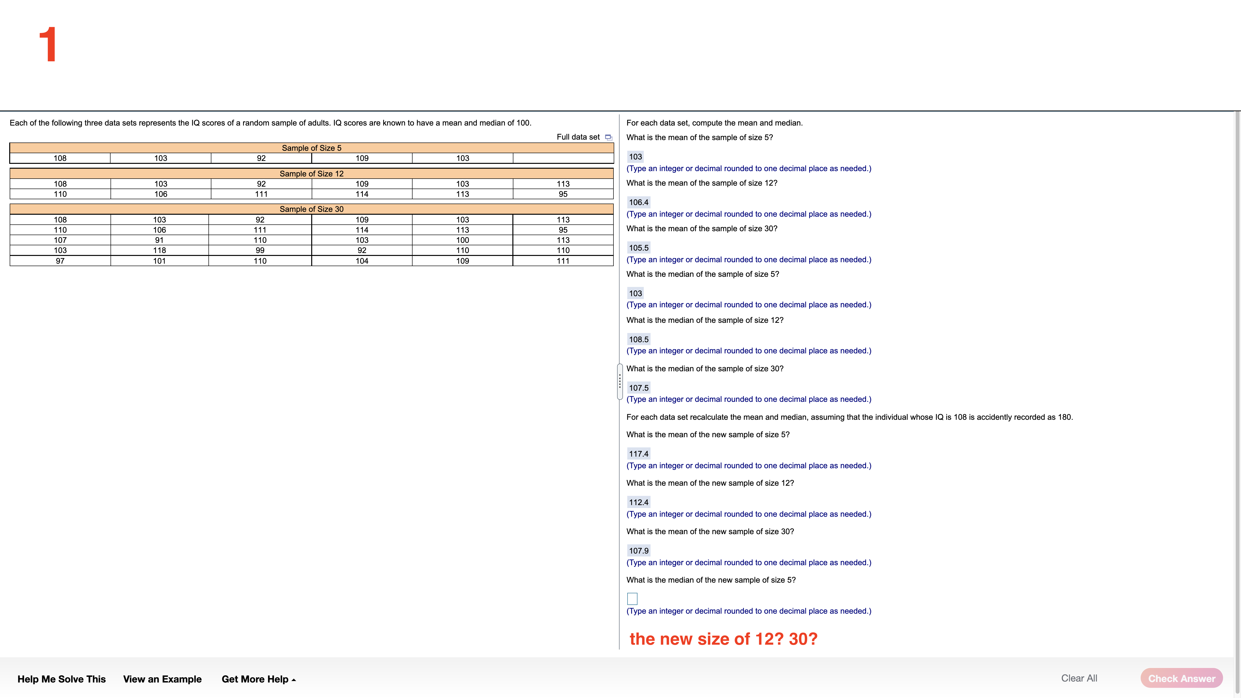
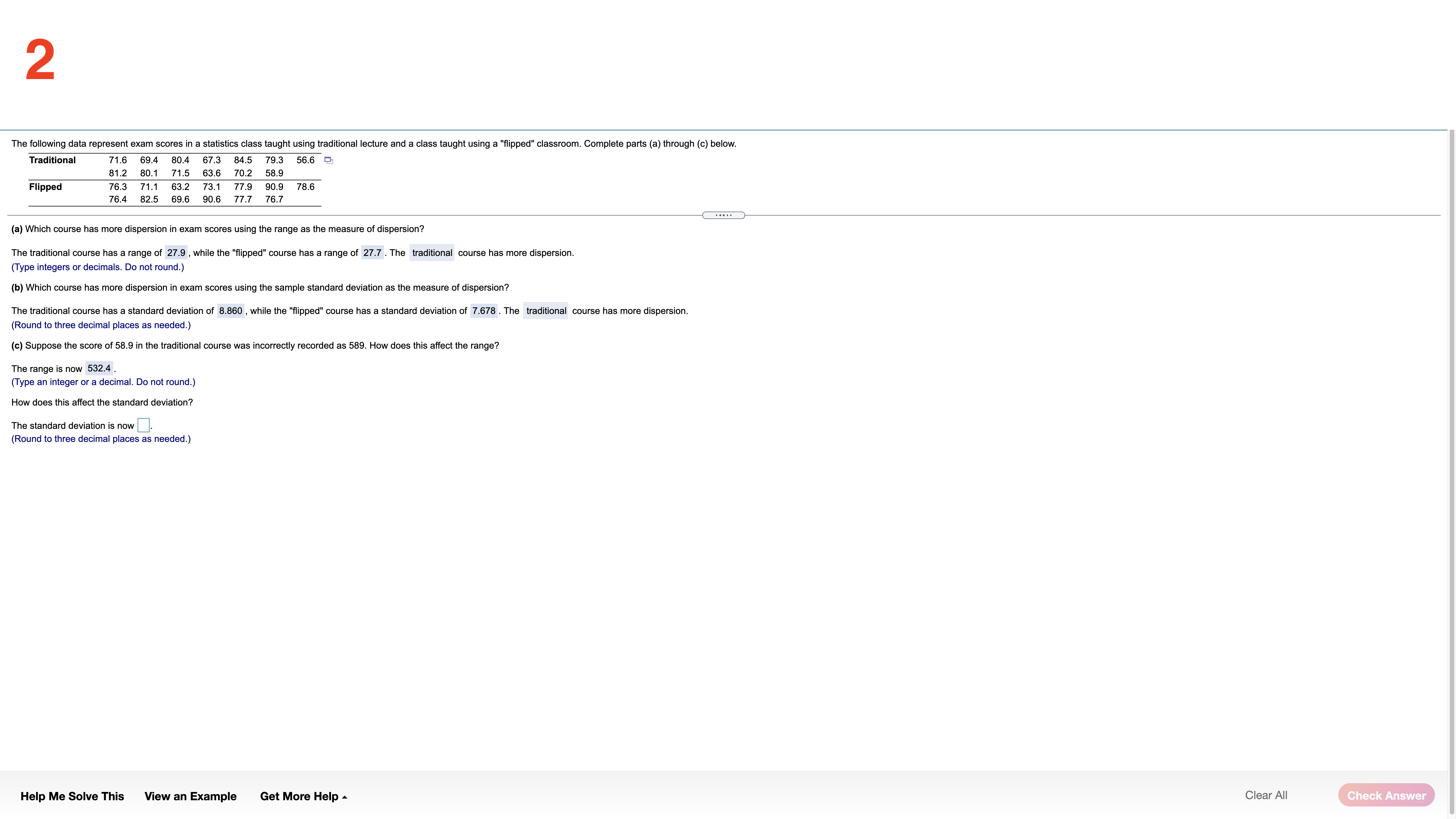
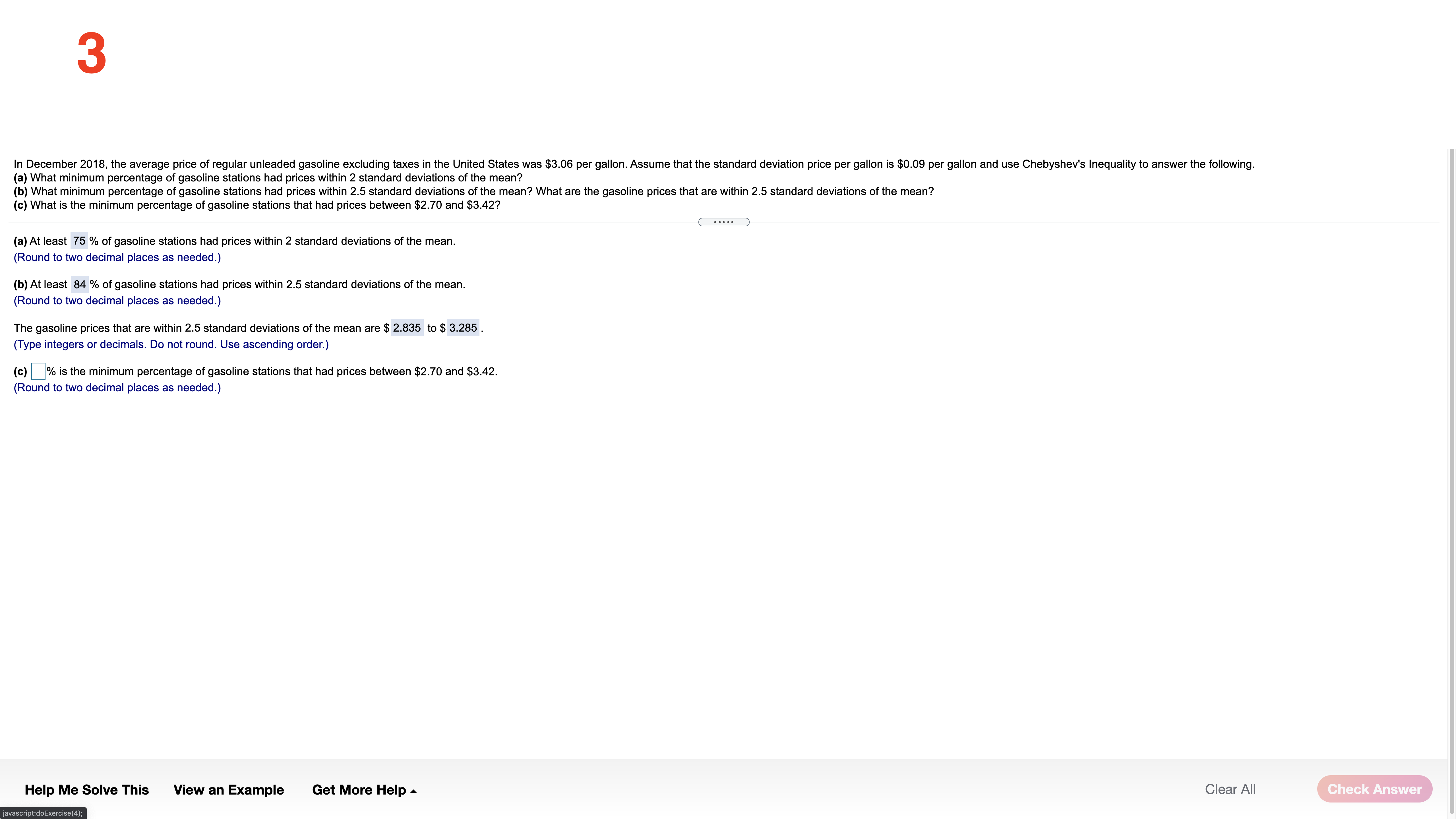
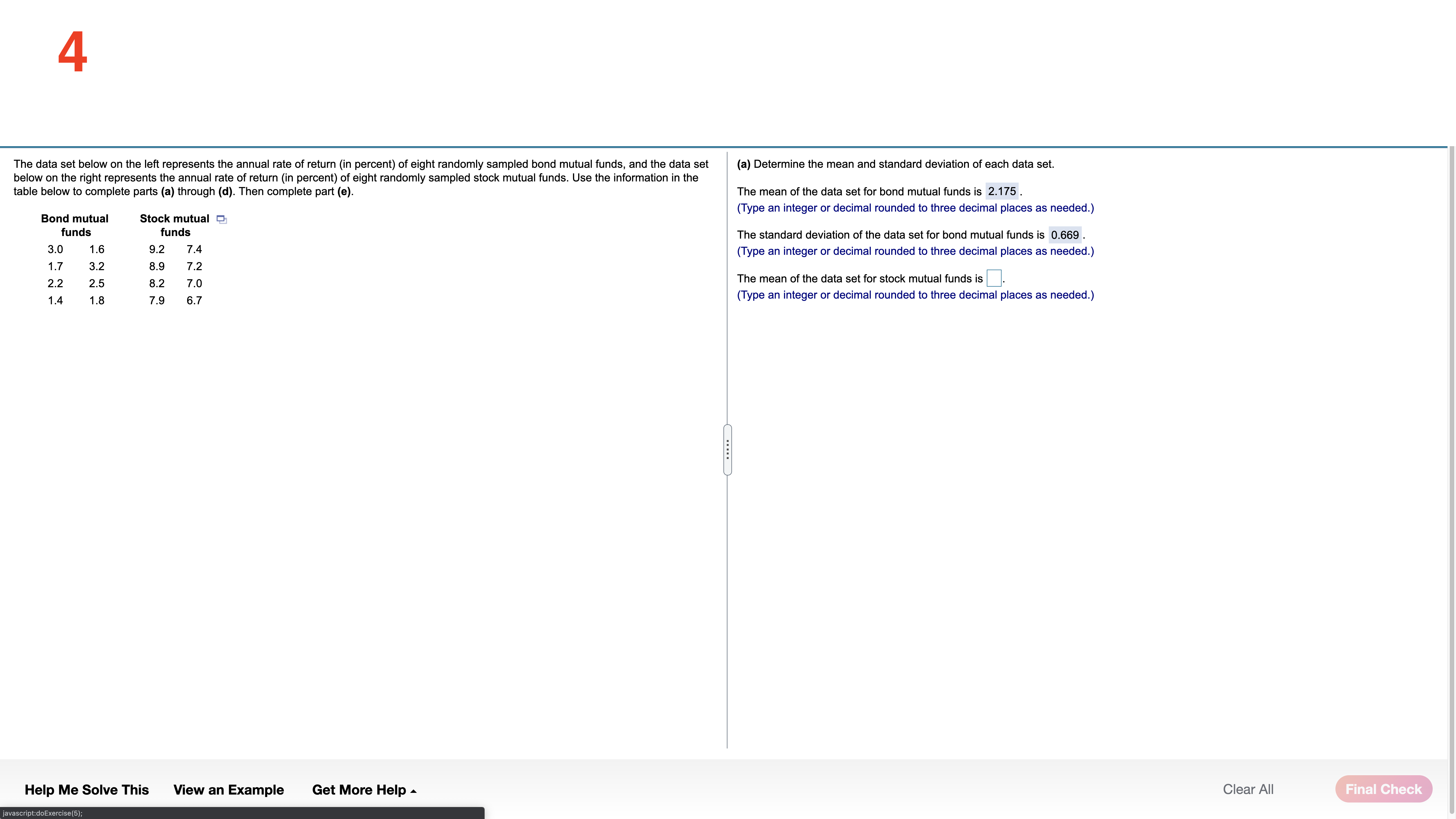
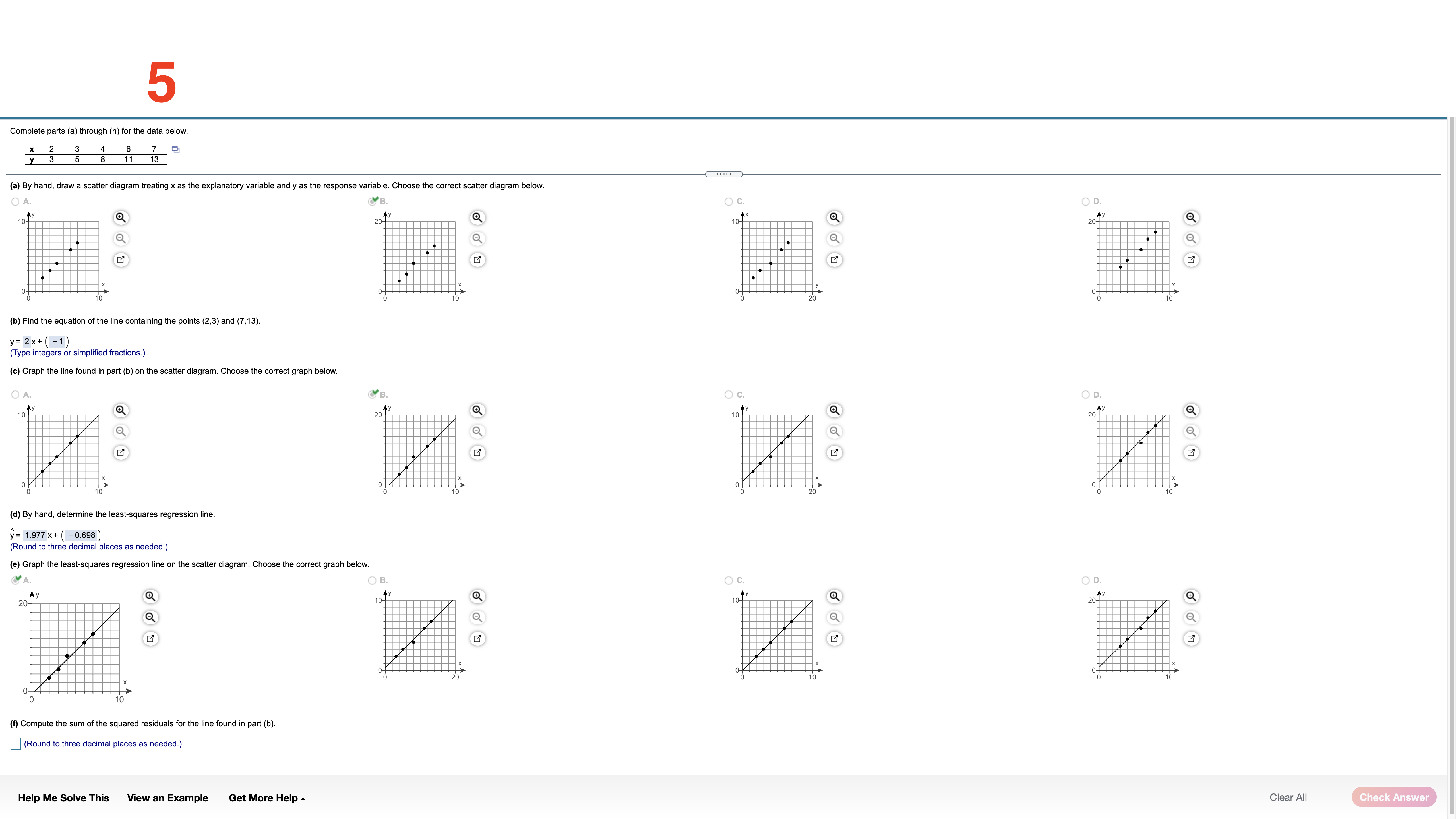
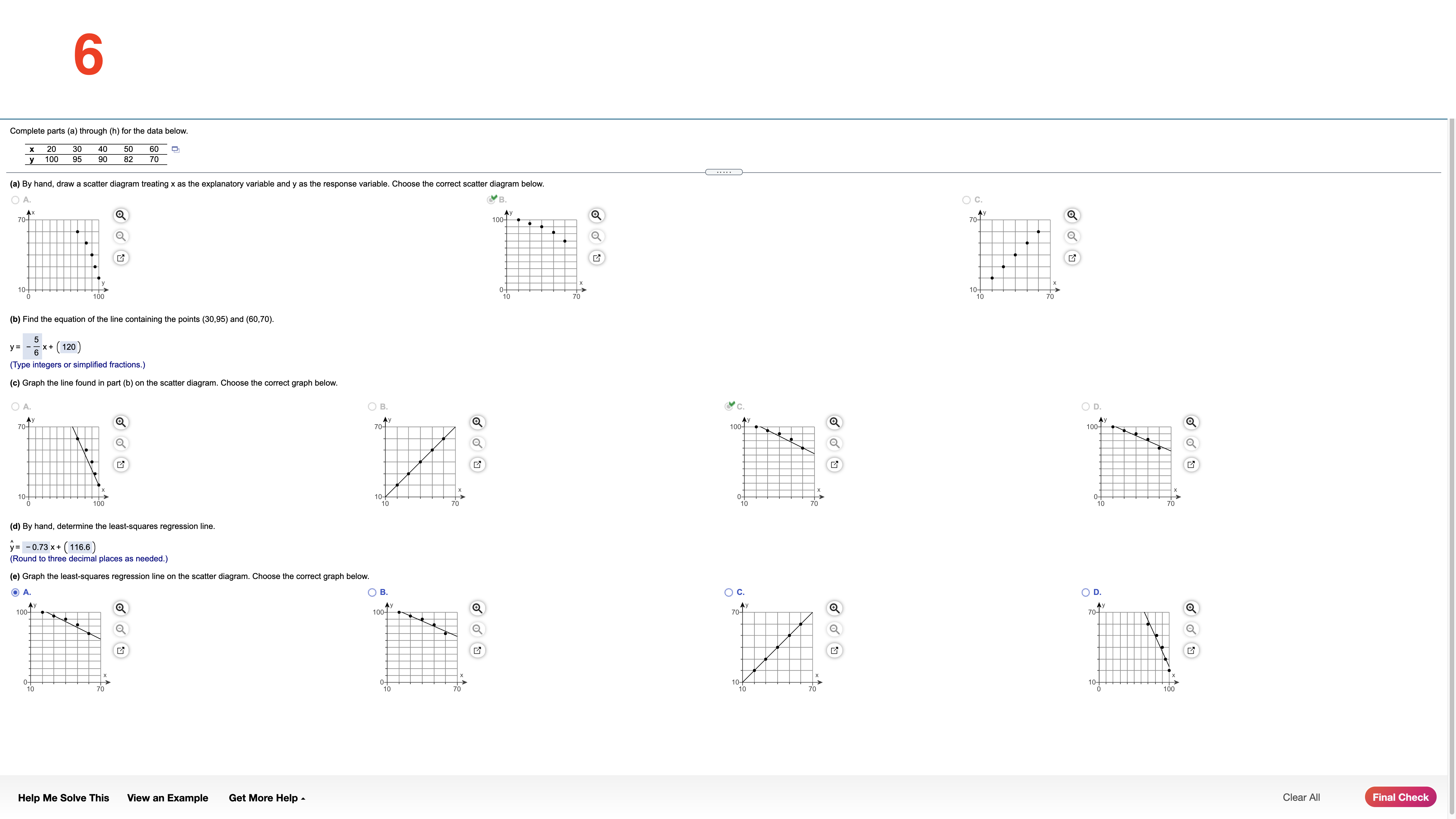
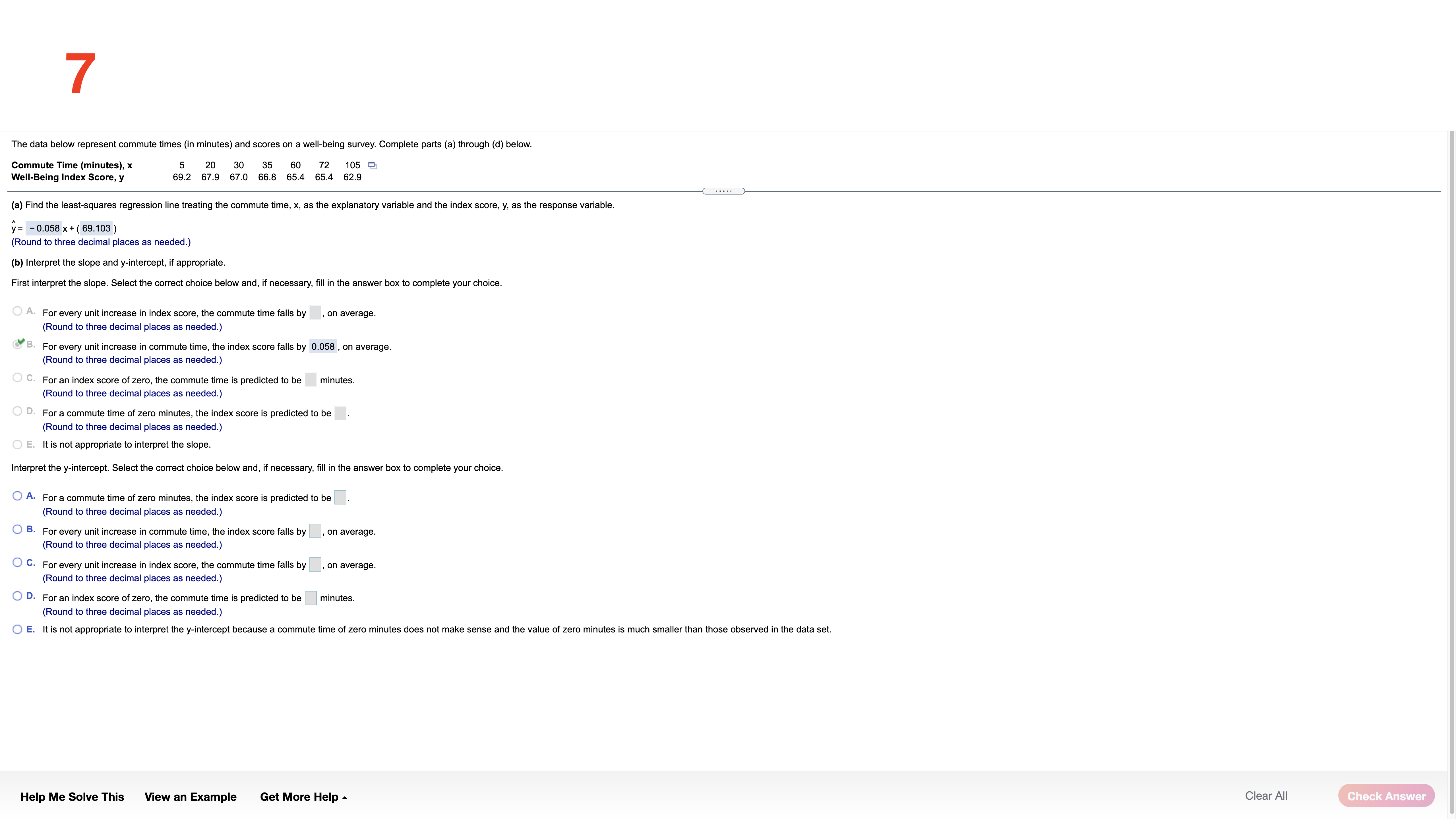
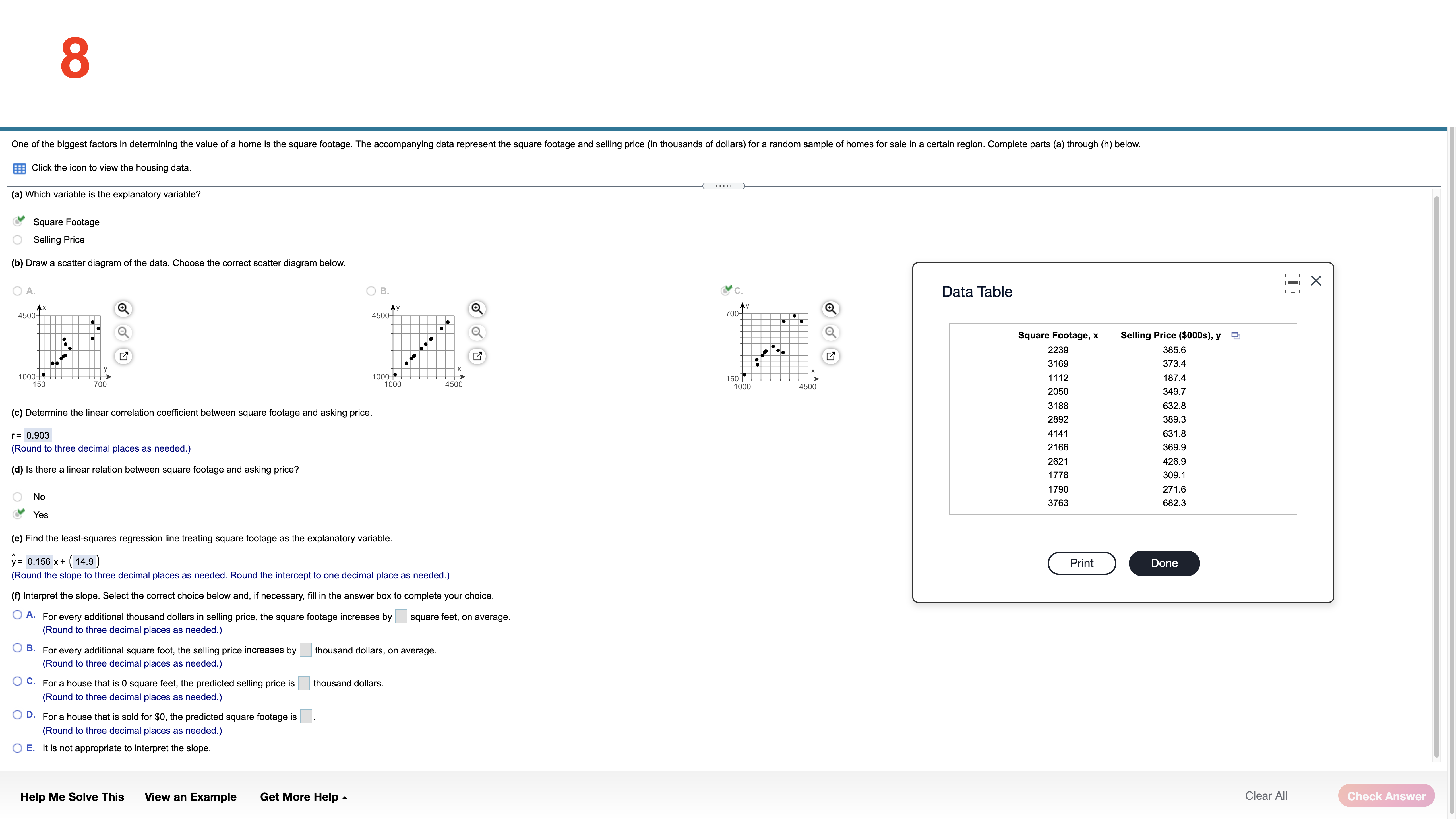
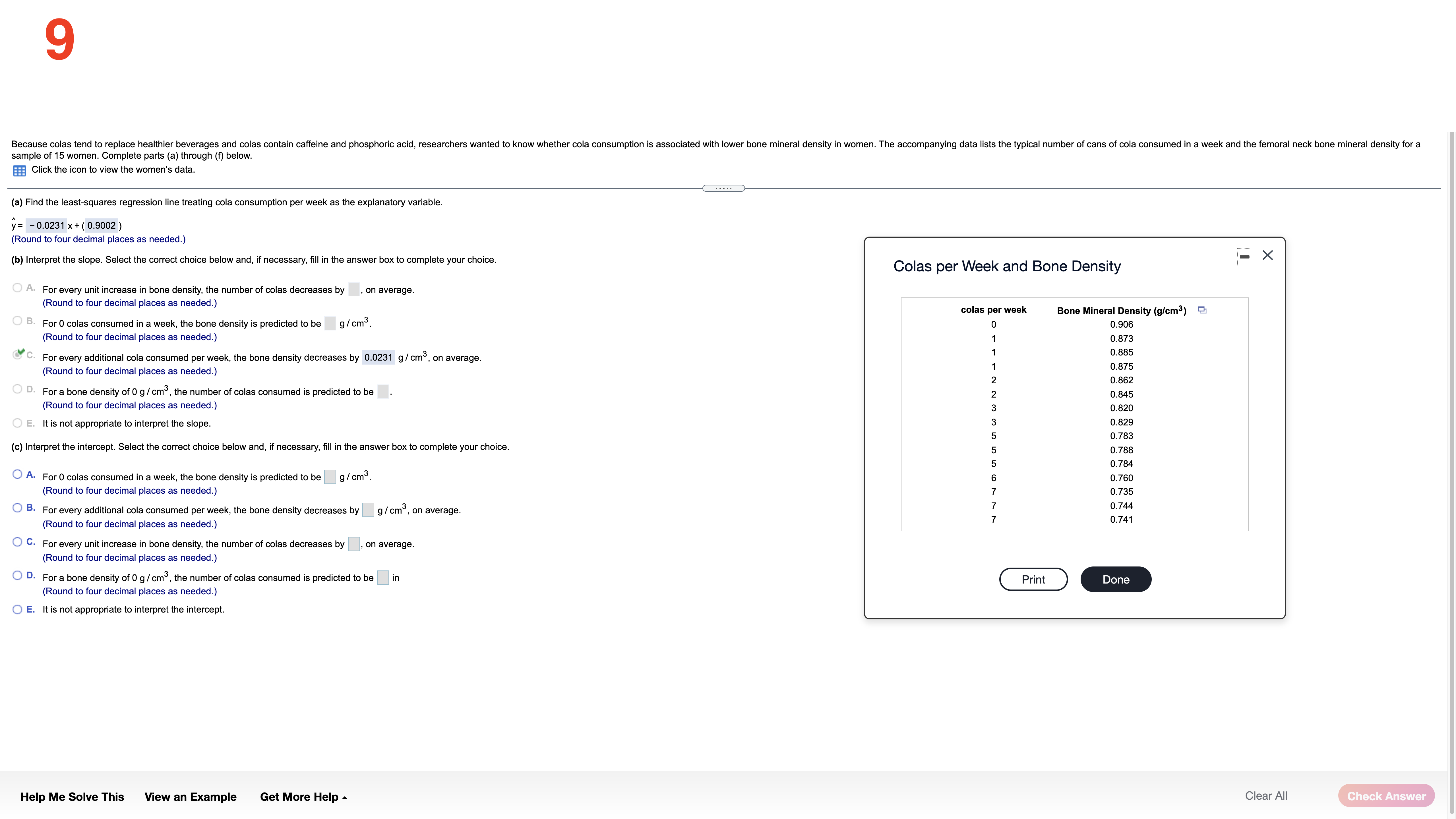
Each of the following three data sets represents the IQ scores of a random sample of adults. IQ scores are known to have a mean and median of 100. For each data set, compute the mean and median. Full data set What is the mean of the sample of size 5? Sample of Size 5 108 103 92 109 103 10 Sample of Size 12 (Type an integer or decimal rounded to one decimal place as needed.) 108 103 92 109 103 113 What is the mean of the sample of size 12? 110 106 11 114 113 95 Sample of Size 30 106.4 108 103 92 109 103 113 (Type an integer or decimal rounded to one decimal place as needed.) 110 106 111 114 113 95 What is the mean of the sample of size 30? 107 91 110 103 100 113 103 118 99 92 110 110 105.5 97 101 110 104 109 111 (Type an integer or decimal rounded to one decimal place as needed.) What is the median of the sample of size 5? 103 (Type an integer or decimal rounded to one decimal place as needed.) What is the median of the sample of size 12? 108.5 (Type an integer or decimal rounded to one decimal place as needed.) What is the median of the sample of size 30? 107.5 (Type an integer or decimal rounded to one decimal place as needed.) For each data set recalculate the mean and median, assuming that the individual whose IQ is 108 is accidently recorded as 180. What is the mean of the new sample of size 5? 117.4 (Type an integer or decimal rounded to one decimal place as needed.) What is the mean of the new sample of size 12? 112.4 (Type an integer or decimal rounded to one decimal place as needed.) What is the mean of the new sample of size 30? 107.9 (Type an integer or decimal rounded to one decimal place as needed.) What is the median of the new sample of size 5? (Type an integer or decimal rounded to one decimal place as needed.) the new size of 12? 30? Help Me Solve This View an Example Get More Help - Clear All Check Answer2 The following data represent exam scores in a statistics class taught using traditional lecture and a class taught using a "flipped" classroom. Complete parts (a) through (c) below. Traditional 71.6 69.4 8 80.4 67.3 84.5 79.3 56.69 81.2 80.1 71.5 63.6 70.2 58.9 Flipped 76.3 71.1 63.2 77.9 90.9 78.6 76.4 82.5 69.6 90.6 77.7 76.7 (a) Which course has more dispersion in exam scores using the range as the measure of dispersion? The traditional course has a range of 27.9 , while the "flipped" course has a range of 27.7 . The traditional course has more dispersion. (Type integers or decimals. Do not round.) (b) Which course has more dispersion in exam scores using the sample standard deviation as the measure of dispersion? The traditional course has a standard deviation of 8.860 , while the "flipped" course has a standard deviation of 7.678 . The traditional course has more dispersion. (Round to three decimal places as needed.) (c) Suppose the score of 58.9 in the traditional course was incorrectly recorded as 589. How does this affect the range? The range is now 532.4 (Type an integer or a decimal. Do not round.) How does this affect the standard deviation? The standard deviation is now Round to three decimal places as needed.) Help Me Solve This View an Example Get More Help - Clear All Check Answer3 In December 2018, the average price of regular unleaded gasoline excluding taxes in the United States was $3.06 per gallon.Assume that the standard deviation price per gallon is $0.09 per gallon and use Chebyshev's Inequality to answer the following. (a) What minimum percentage of gasoline stations had prices within 2 standard deviations of the mean? (b) What minimum percentage of gasoline stations had prices within 2.5 standard deviations of the mean? What are the gasoline prices that are within 2.5 standard deviations of the mean? (c) What is the minimum percentage ofgasoline stations that had prices between $2.70 and $3.42? (a) At least 75 \"A of gasoline stations had prices within 2 standard deviations ofthe mean. (Round to two decimal places as needed.) (b) At least 84 \"In of gasoline stations had prices within 2.5 standard deviations of the mean. (Round to two decimal places as needed.) The gasoline prices that are within 2.5 standard deviations of the mean are $ 2.835 to $ 3.285 . (Type integers or decimals. Do not round. Use ascending order.) (c) % is the minimum percentage ofgasoline stations that had prices between $2.70 and $3.42. (Round to two decimal places as needed.) Help Me Solve This View an Example Get More Help A Clear All _ 4 The data set below on the left represents the annual rate of return (in percent) oteight randomly sampled bond mutual funds, and the data set (a) Determine the mean and standard deviation of each data set. below on the right represents the annual rate of return (in percent) at eight randomly sampled stock mutual funds. Use the information in the table below tn complete parts (a) through (d). Then complete part (e). The mean 01 the data set for bond mutual funds is 2.175 . (Type an integer or decimal rounded to three decimal places as needed.) Bond mutual Stock mutual :1: fund! NM! The standard deviation of the data set for bond mutual funds is 0,669 . 3-0 1-5 9-2 7-4 (Type an integer or decimal rounded to three decimal places as needed.) 1.7 3.2 8.9 7.2 2,2 25 8.2 70 The mean of the data set for stock mutual funds is . 1.4 1.6 7.9 6.7 (Type an integer or decimal rounded to three decimal places as needed.) Help Me Solve This View an Example Get More Help A Clear All 5 Complete parts (a) through (h) for the data below. y 3 5 8 11 13 (a) By hand, draw a scatter diagram treating x as the explanatory variable and y as the response variable. Choose the correct scatter diagram below. O A B OD 10- 20- O (b) Find the equation of the line containing the points (2,3) and (7, 13). y= 2 x + (- 1) (Type integers or simplified fractions.) (c) Graph the line found in part (b) on the scatter diagram. Choose the correct graph below. OA B C. OD 20- 10-1 (d) By hand, determine the least-squares regression line. y= 1.977 x + (-0.698 (Round to three decimal places as needed.) (e) Graph the least-squares regression line on the scatter diagram. Choose the correct graph below. B C. OD 20- 10- 10- 20- (f) Compute the sum of the squared residuals for the line found in part (b). (Round to three decimal places as needed.) Help Me Solve This View an Example Get More Help - Clear All Check Answer6 Complete parts (a) through (h) for the data below. 20 40 50 60 y 100 95 90 82 70 (a) By hand, draw a scatter diagram treating x as the explanatory variable and y as the response variable. Choose the correct scatter diagram below. O A B. C. 100- 70- 70 10% (b) Find the equation of the line containing the points (30,95) and (60,70). y= - 6 X+ (120 ) (Type integers or simplified fractions.) (c) Graph the line found in part (b) on the scatter diagram. Choose the correct graph below. OA OB C. OD 100T 100- 10- (d) By hand, determine the least-squares regression line. y= -0.73 x+ (116.6 ) (Round to three decimal places as needed.) (e) Graph the least-squares regression line on the scatter diagram. Choose the correct graph below. OA B. OD 100- 100 My 701 70 70 Help Me Solve This View an Example Get More Help - Clear All Final CheckThe data below represent commute times (in minutes) and scores on a well-being survey. Complete parts (a) through (d) below. Commute Time (minutes), x 5 20 30 35 60 72 105 Well-Being Index Score, y 69.2 67.9 67.0 66.8 65.4 65.4 62.9 . . . . (a) Find the least-squares regression line treating the commute time, x, as the explanatory variable and the index score, y, as the response variable. y= - 0.058 x + ( 69.103 ) (Round to three decimal places as needed.) (b) Interpret the slope and y-intercept, if appropriate First interpret the slope. Select the correct choice below and, if necessary, fill in the answer box to complete your choice. O A. For every unit increase in index score, the commute time falls by , on average. Round to three decimal places as needed.) For every unit increase in commute time, the index score falls by 0.058 , on average. Round to three decimal places as needed.) O C. For an index score of zero, the commute time is predicted to be minutes. (Round to three decimal places as needed.) O D. For a commute time of zero minutes, the index score is predicted to be (Round to three decimal places as needed.) O E. It is not appropriate to interpret the slope Interpret the y-intercept. Select the correct choice below and, if necessary, fill in the answer box to complete your choice. O A. For a commute time of zero minutes, the index score is predicted to be Round to three decimal places as needed.) O B. For every unit increase in commute time, the index score falls by , on average. Round to three decimal places as needed.) O C. For every unit increase in index score, the commute time falls by , on average. (Round to three decimal places as needed.) O D. For an index score of zero, the commute time is predicted to be |minutes. (Round to three decimal places as needed.) O E. It is not appropriate to interpret the y-intercept because a commute time of zero minutes does not make sense and the value of zero minutes is much smaller than those observed in the data set. Help Me Solve This View an Example Get More Help - Clear All Check Answer8 One of the biggest factors in determining the value of a home is the square footage. The accompanying data represent the square footage and selling price (in thousands of dollars) for a random sample of homes for sale in a certain region. Complete parts (a) through (h) below. Click the icon to view the housing data. (a) Which variable is the explanatory variable? Square Footage Selling Price (b) Draw a scatter diagram of the data. Choose the correct scatter diagram below. X OA O B. VC. Data Table AX 4500- 700 4500- Square Footage, x Selling Price ($000s), y 2239 385.6 3169 373.4 000 1000- 700 1000 4500 50- 150 111 187. 1000 4500 2050 349.7 3188 632. (c) Determine the linear correlation coefficient between square footage and asking price. 2892 389.3 r= 0.903 4141 $31.8 (Round to three decimal places as needed.) 2166 369.9 2621 426.9 (d) Is there a linear relation between square footage and asking price? 1778 309.1 1790 O 271.6 No 3763 682.3 Yes (e) Find the least-squares regression line treating square footage as the explanatory variable. y= 0.156 x + (14.9) Print Done (Round the slope to three decimal places as needed. Round the intercept to one decimal place as needed.) (f) Interpret the slope. Select the correct choice below and, if necessary, fill in the answer box to complete your choice. O A. For every additional thousand dollars in selling price, the square footage increases by square feet, on average. Round to three decimal places as needed.) O B. For every additional square foot, the selling price increases by |thousand dollars, on average. Round to three decimal places as needed.) O C. For a house that is 0 square feet, the predicted selling price is thousand dollars. (Round to three decimal places as needed.) O D. For a house that is sold for $0, the predicted square footage is (Round to three decimal places as needed.) O E. It is not appropriate to interpret the slope. Help Me Solve This View an Example Get More Help - Clear All Check Answer9 Because colas tend to replace healthier beverages and colas contain caffeine and phosphoric acid, researchers wanted to know whether cola consumption is associated with lower bone mineral density in women. The accompanying data lists the typical number of cans of cola consumed in a week and the femoral neck bone mineral density for a sample of 15 women. Complete parts (a) through (f) below. Click the icon to view the women's data. (a) Find the least-squares regression line treating cola consumption per week as the explanatory variable. y= -0.0231 x + ( 0.9002 ) (Round to four decimal places as needed.) (b) Interpret the slope. Select the correct choice below and, if necessary, fill in the answer box to complete your choice. - X Colas per Week and Bone Density O A. For every unit increase in bone density, the number of colas decreases by , on average. Round to four decimal places as needed.) colas per week Bone Mineral Density (g/cm3) O B. For 0 colas consumed in a week, the bone density is predicted to be g/ cm3. 0.906 (Round to four decimal places as needed. 0.873 SC. F 0.885 . For every additional cola consumed per week, the bone density decreases by 0.0231 g/ cm, on average. (Round to four decimal places as needed.) 0.875 0.862 O D. For a bone density of 0 g / cm, the number of colas consumed is predicted to be 0.845 (Round to four decimal places as needed.) 0.820 O E. It is not appropriate to interpret the slope. .829 0.783 VVVOMICIDI W W N N- (c) Interpret the intercept. Select the correct choice below and, if necessary, fill in the answer box to complete your choice. 0.788 0.784 A. For 0 colas consumed in a week, the bone density is predicted to be g/ cm3. 0.760 (Round to four decimal places as needed.) 0.735 O B. For every additional cola consumed per week, the bone density decreases by g/ cm, on average. 0.744 0.741 (Round to four decimal places as needed.) O C. For every unit increase in bone density, the number of colas decreases by , on average. Round to four decimal places as needed.) O D. For a bone density of 0 g / cm, the number of colas consumed is predicted to be in Print Done (Round to four decimal places as needed.) O E. It is not appropriate to interpret the intercept. Help Me Solve This View an Example Get More Help - Clear All Check