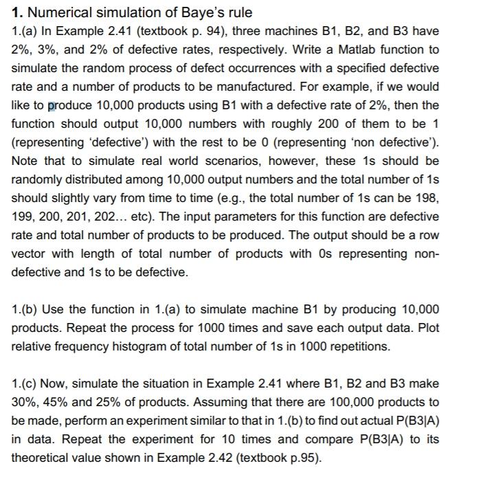
neet matlab code thx

1. Numerical simulation of Baye's rule 1.(a) In Example 2.41 (textbook p. 94), three machines B1, B2, and B3 have 2%, 3%, and 2% of defective rates, respectively. Write a Matlab function to simulate the random process of defect occurrences with a specified defective rate and a number of products to be manufactured. For example, if we would like to produce 10,000 products using B1 with a defective rate of 2%, then the function should output 10,000 numbers with roughly 200 of them to be 1 (representing 'defective') with the rest to be 0 (representing 'non defective'). Note that to simulate real world scenarios, however, these 1s should be randomly distributed among 10,000 output numbers and the total number of 1s should slightly vary from time to time (e.g., the total number of 1s can be 198, 199, 200, 201, 202... etc). The input parameters for this function are defective rate and total number of products to be produced. The output should be a row vector with length of total number of products with Os representing non- defective and 1s to be defective. 1.(b) Use the function in 1.(a) to simulate machine B1 by producing 10,000 products. Repeat the process for 1000 times and save each output data. Plot relative frequency histogram of total number of 1s in 1000 repetitions. 1.(C) Now, simulate the situation in Example 2.41 where B1, B2 and B3 make 30%, 45% and 25% of products. Assuming that there are 100,000 products to be made, perform an experiment similar to that in 1.(b) to find out actual P(B3|A) in data. Repeat the experiment for 10 times and compare P(B3A) to its theoretical value shown in Example 2.42 (textbook p.95). 1. Numerical simulation of Baye's rule 1.(a) In Example 2.41 (textbook p. 94), three machines B1, B2, and B3 have 2%, 3%, and 2% of defective rates, respectively. Write a Matlab function to simulate the random process of defect occurrences with a specified defective rate and a number of products to be manufactured. For example, if we would like to produce 10,000 products using B1 with a defective rate of 2%, then the function should output 10,000 numbers with roughly 200 of them to be 1 (representing 'defective') with the rest to be 0 (representing 'non defective'). Note that to simulate real world scenarios, however, these 1s should be randomly distributed among 10,000 output numbers and the total number of 1s should slightly vary from time to time (e.g., the total number of 1s can be 198, 199, 200, 201, 202... etc). The input parameters for this function are defective rate and total number of products to be produced. The output should be a row vector with length of total number of products with Os representing non- defective and 1s to be defective. 1.(b) Use the function in 1.(a) to simulate machine B1 by producing 10,000 products. Repeat the process for 1000 times and save each output data. Plot relative frequency histogram of total number of 1s in 1000 repetitions. 1.(C) Now, simulate the situation in Example 2.41 where B1, B2 and B3 make 30%, 45% and 25% of products. Assuming that there are 100,000 products to be made, perform an experiment similar to that in 1.(b) to find out actual P(B3|A) in data. Repeat the experiment for 10 times and compare P(B3A) to its theoretical value shown in Example 2.42 (textbook p.95)