Answered step by step
Verified Expert Solution
Question
1 Approved Answer
Next, redefine the Lookup function to classify employees as Above Average and Below Average based on whether they scored above or below an average of

Next, redefine the Lookup function to classify employees as Above Average and Below Average based on whether they scored above or below an average of 5 in their three performance scores. Place the results in the 7th Column, or Column G. (can someone explain to me how this formula is typed) i HAVE THIS =LOOKUP(E2,{0,6,10},{"Below Average","Above Average"}) should the number be a 5 or a 6.
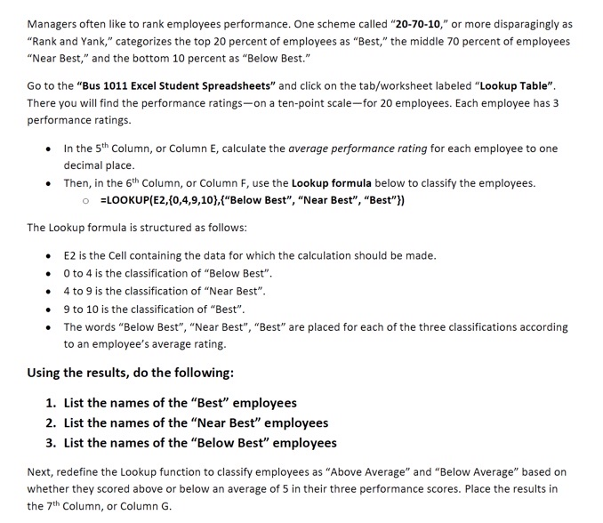
Managers often like to rank employees performance. One scheme called "20-70-10," or more disparagingly as "Rank and Yank,"categorizes the top 20 percent of employees as "Best," the middle 70 percent of employees "Near Best," and the bottom 10 percent as "Below Best." Go to the "Bus 1011 Excel Student Spreadsheets" and click on the tab/worksheet labeled "Lookup Table". There you will find the performance ratings-on a ten-point scale-for 20 employees. Each employee has 3 performance ratings. In the 5th Column, or Column E, calculate the average performance rating for each employee to one decimal place. Then, in the 6th Column, or Column F, use the Lookup formula below to classify the employees. o =LOOKUP(E2,{0,4,9,10},{"Below Best", "Near Best", "Best"}) The Lookup formula is structured as follows: E2 is the Cell containing the data for which the calculation should be made. Oto 4 is the classification of "Below Best". 4 to 9 is the classification of "Near Best". 9 to 10 is the classification of "Best". The words "Below Best", "Near Best", "Best" are placed for each of the three classifications according to an employee's average rating. Using the results, do the following: 1. List the names of the "Best" employees 2. List the names of the "Near Best" employees 3. List the names of the "Below Best" employees Next, redefine the Lookup function to classify employees as "Above Average" and "Below Average" based on whether they scored above or below an average of 5 in their three performance scores. Place the results in the 7th Column, or Column G. Managers often like to rank employees performance. One scheme called "20-70-10," or more disparagingly as "Rank and Yank,"categorizes the top 20 percent of employees as "Best," the middle 70 percent of employees "Near Best," and the bottom 10 percent as "Below Best." Go to the "Bus 1011 Excel Student Spreadsheets" and click on the tab/worksheet labeled "Lookup Table". There you will find the performance ratings-on a ten-point scale-for 20 employees. Each employee has 3 performance ratings. In the 5th Column, or Column E, calculate the average performance rating for each employee to one decimal place. Then, in the 6th Column, or Column F, use the Lookup formula below to classify the employees. o =LOOKUP(E2,{0,4,9,10},{"Below Best", "Near Best", "Best"}) The Lookup formula is structured as follows: E2 is the Cell containing the data for which the calculation should be made. Oto 4 is the classification of "Below Best". 4 to 9 is the classification of "Near Best". 9 to 10 is the classification of "Best". The words "Below Best", "Near Best", "Best" are placed for each of the three classifications according to an employee's average rating. Using the results, do the following: 1. List the names of the "Best" employees 2. List the names of the "Near Best" employees 3. List the names of the "Below Best" employees Next, redefine the Lookup function to classify employees as "Above Average" and "Below Average" based on whether they scored above or below an average of 5 in their three performance scores. Place the results in the 7th Column, or Column GStep by Step Solution
There are 3 Steps involved in it
Step: 1

Get Instant Access to Expert-Tailored Solutions
See step-by-step solutions with expert insights and AI powered tools for academic success
Step: 2

Step: 3

Ace Your Homework with AI
Get the answers you need in no time with our AI-driven, step-by-step assistance
Get Started


