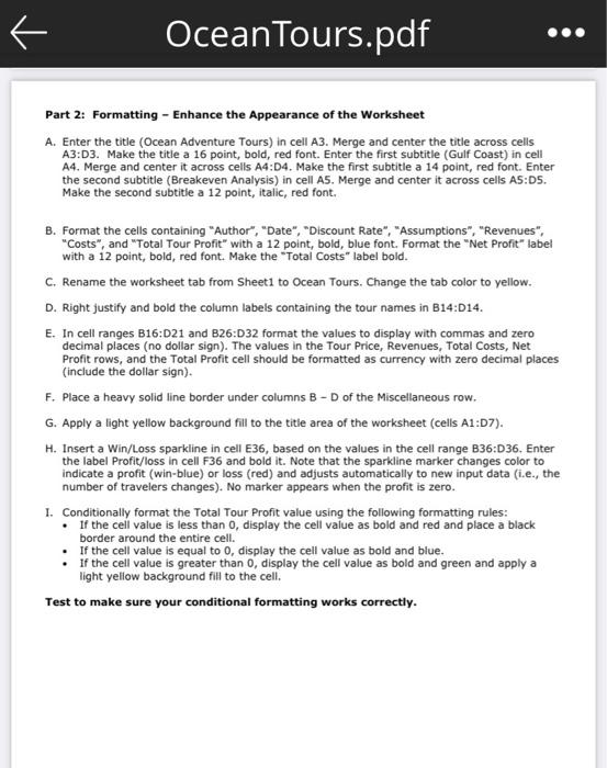
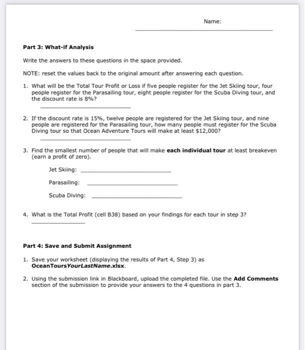
+ Ocean Tours.pdf Part 2: Formatting - Enhance the Appearance of the Worksheet A. Enter the title (Ocean Adventure Tours) in cell A3. Merge and center the title across cells A3:03. Make the title a 16 point, bold, red font. Enter the first subtitle (Gulf Coast) in cell A4. Merge and center it across cells A4:04. Make the first subtitle a 14 point, red font. Enter the second subtitle (Breakeven Analysis) in cell A5. Merge and center it across cells A5:05. Make the second subtitle a 12 point, italic, red font. B. Format the cells containing "Author", "Date", "Discount Rate", "Assumptions", "Revenues", "Costs", and "Total Tour Profit" with a 12 point, bold, blue font. Format the "Net Profit" label with a 12 point, bold, red font. Make the "Total Costs" label bold. C. Rename the worksheet tab from Sheet1 to Ocean Tours, Change the tab color to yellow. D. Right justify and bold the column labels containing the tour names in B14:014. E. In cell ranges B16:021 and B26:032 format the values to display with commas and zero decimal places (no dollar sign). The values in the Tour Price, Revenues, Total Costs, Net Profit rows, and the Total Profit cell should be formatted as currency with zero decimal places (include the dollar sign). F. Place a heavy solid line border under columns B-D of the Miscellaneous row. G. Apply a light yellow background fill to the title area of the worksheet (cells A1:07). H. Insert a Win/Loss sparkline in cell E36, based on the values in the cell range B36:D36. Enter the label Profit/loss in cell F36 and bold it. Note that the sparkline marker changes color to indicate a profit (win-blue) or loss (red) and adjusts automatically to new input data (i.e., the number of travelers changes). No marker appears when the profit is zero. I. Conditionally format the Total Tour Profit value using the following formatting rules: . If the cell value is less than 0, display the cell value as bold and red and place a black border around the entire cell. . If the cell value is equal to 0, display the cell value as bold and blue. If the cell value is greater than o, display the cell value as bold and green and apply a light yellow background fill to the cell. Test to make sure your conditional formatting works correctly. Name: Part 3: What-if Analysis Write the answers to these questions in the space provided. NOTE: reset the values back to the original amount after answering each question. 1. What will be the Total Tour Profit or Loss if five people register for the Jet Skiing tour, four people register for the Parasailing tour, eight people register for the Scuba Diving tour, and the discount rate is 8%? 2. If the discount rate is 15%, twelve people are registered for the Jet Skiing tour, and nine people are registered for the Parasailing tour, how many people must register for the Scuba Diving tour so that Ocean Adventure Tours will make at least $12,000? 3. Find the smallest number of people that will make each individual tour at least breakeven (earn a profit of zero). Jet Skiing: Parasailing: Scuba Diving: 4. What is the Total Profit (cell B38) based on your findings for each tour in step 3? Part 4: Save and Submit Assignment 1. Save your worksheet (displaying the results of Part 4, Step 3) as Ocean Tours YourLastName.xlsx. 2. Using the submission link in Blackboard, upload the completed file. Use the Add Comments section of the submission to provide your answers to the 4 questions in part 3


