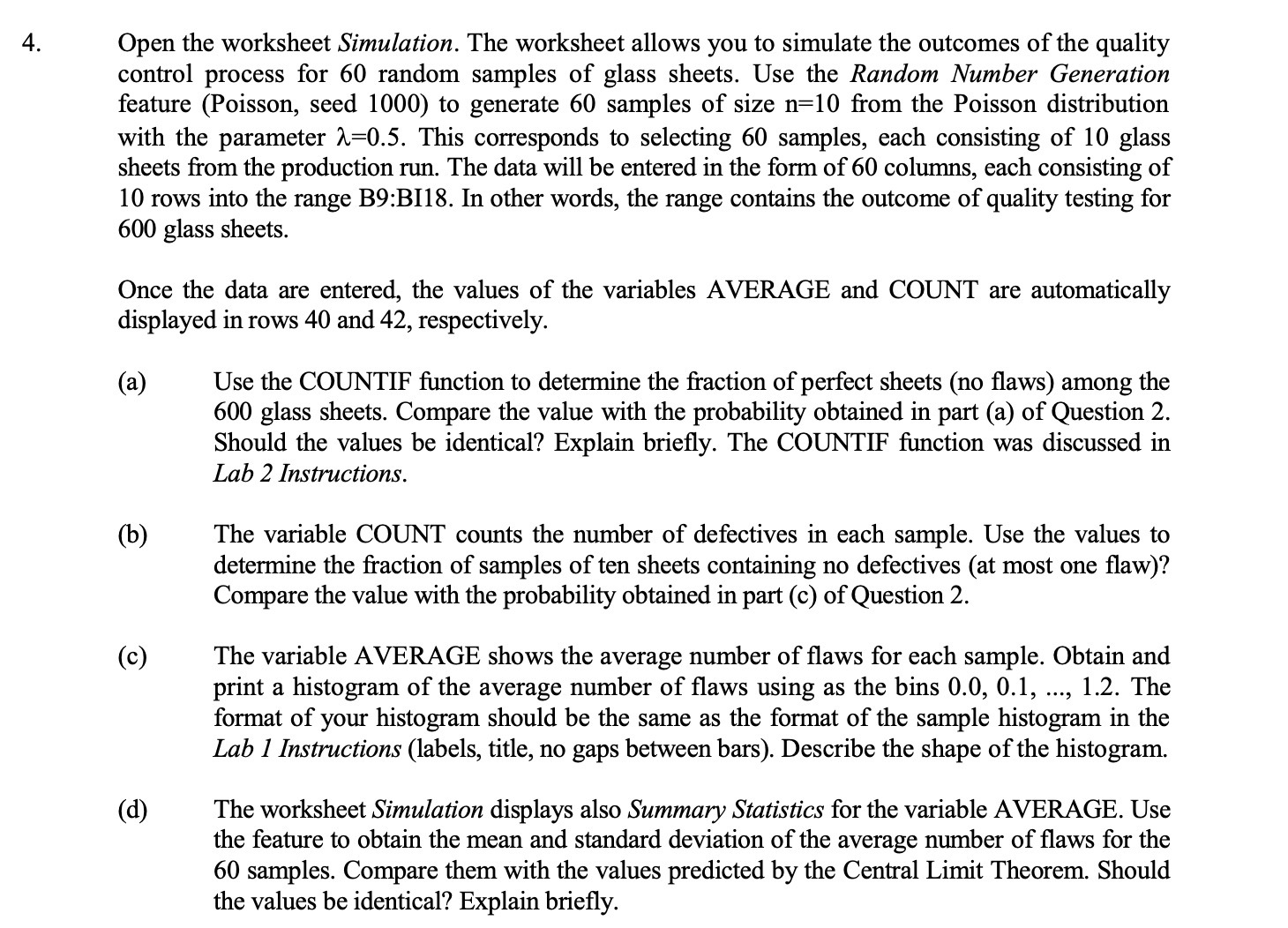
Open the worksheet Simulation. The worksheet allows you to simulate the outcomes of the quality control process for 60 random samples of glass sheets. Use the Random Number Generation feature (Poisson, seed 1000) to generate 60 samples of size n=10 'om the Poisson distribution with the parameter l=0.5. This corresponds to selecting 60 samples, each consisting of 10 glass sheets from the production run. The data will be entered in the form of 60 columns, each consisting of 10 rows into the range B92B118. In other words, the range contains the outcome of quality testing for 600 glass sheets. Once the data are entered, the values of the variables AVERAGE and COUNT are automatically displayed in rows 40 and 42, respectively. (a) Use the COUNTIF function to determine the fraction of perfect sheets (no aws) among the 600 glass sheets. Compare the value with the probability obtained in part (a) of Question 2. Should the values be identical? Explain briey. The COUNTIF function was discussed in Lab 2 Instructions. (b) The variable COUNT counts the number of defectives in each sample. Use the values to determine the fraction of samples of ten sheets containing no defectives (at most one aw)? Compare the value with the probability obtained in part (c) of Question 2. (c) The variable AVERAGE shows the average number of aws for each sample. Obtain and print a histogram of the average number of aws using as the bins 0.0, 0.1, ..., 1.2. The format of your histogram should be the same as the format of the sample histogram in the Lab 1 Instructions (labels, title, no gaps between bars). Describe the shape of the histogram. (d) The worksheet Simulation displays also Summary Statistics for the variable AVERAGE. Use the feature to obtain the mean and standard deviation of the average number of aws for the 60 samples. Compare them with the values predicted by the Central Limit Theorem. Should the values be identical? Explain briey