Question
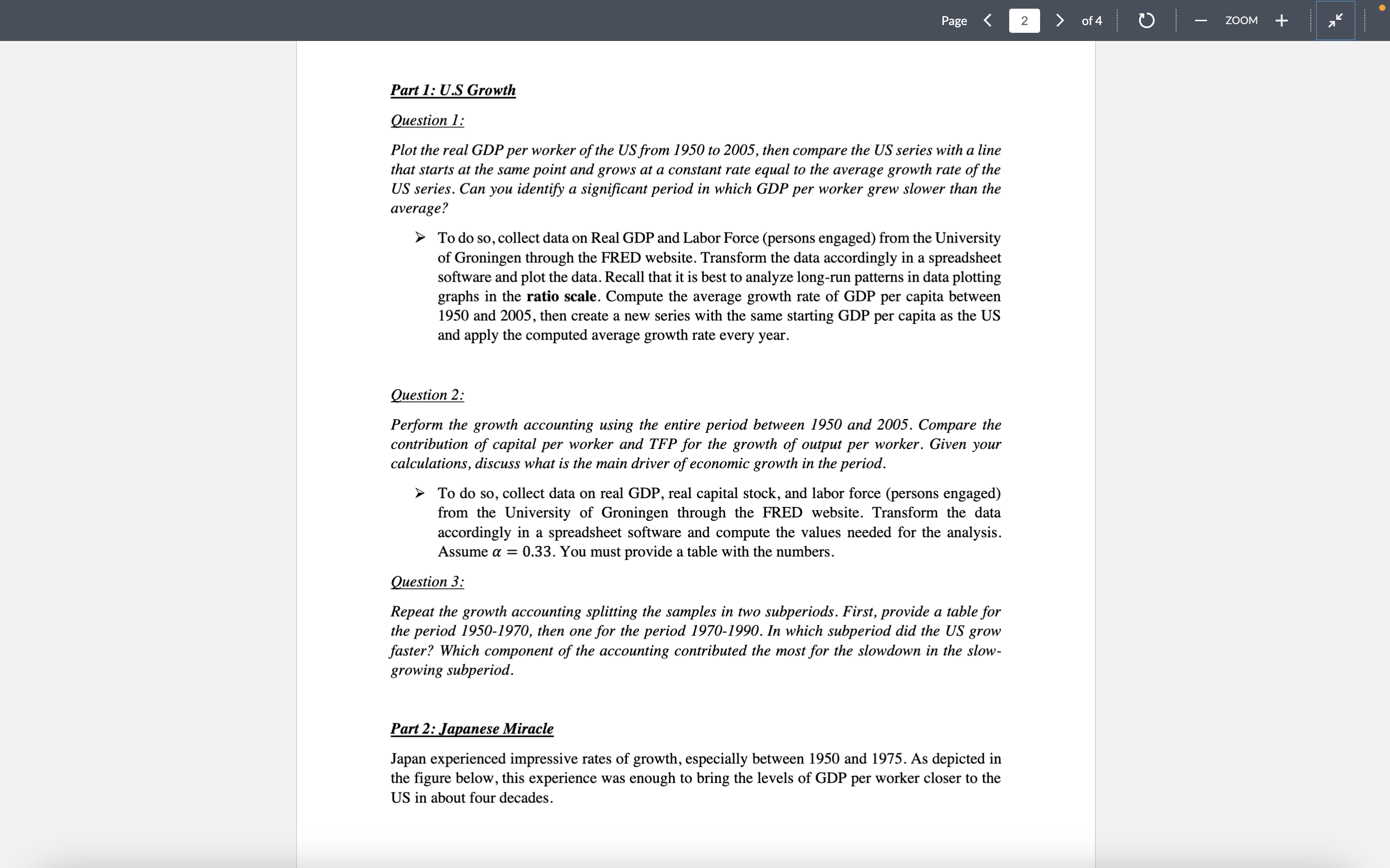
Part 1: U.S Growth Question 1: Plot the real GDP per worker of the US from 1950 to 2005, then compare the US series with


Part 1: U.S Growth Question 1: Plot the real GDP per worker of the US from 1950 to 2005, then compare the US series with a line that starts at the same point and grows at a constant rate equal to the average growth rate of the US series. Can you identify a significant period in which GDP per worker grew slower than the average? ? To do so, collect data on Real GDP and Labor Force (persons engaged) from the University of Groningen through the FRED website. Transform the data accordingly in a spreadsheet software and plot the data. Recall that it is best to analyze long-run patterns in data plotting graphs in the ratio scale. Compute the average growth rate of GDP per capita between 1950 and 2005, then create a new series with the same starting GDP per capita as the US and apply the computed average growth rate every year.
Question 2: Perform the growth accounting using the entire period between 1950 and 2005. Compare the contribution of capital per worker and TFP for the growth of output per worker. Given your calculations, discuss what is the main driver of economic growth in the period. ? To do so, collect data on real GDP, real capital stock, and labor force (persons engaged) from the University of Groningen through the FRED website. Transform the data accordingly in a spreadsheet software and compute the values needed for the analysis. Assume ? = 0.33. You must provide a table with the numbers.
Question 3: Repeat the growth accounting splitting the samples in two subperiods. First, provide a table for the period 1950-1970, then one for the period 1970-1990. In which subperiod did the US grow faster? Which component of the accounting contributed the most for the slowdown in the slow- growing subperiod
. Use This Link For Question #1 - https://fred.stlouisfed.org/series/A939RX0Q048SBEA
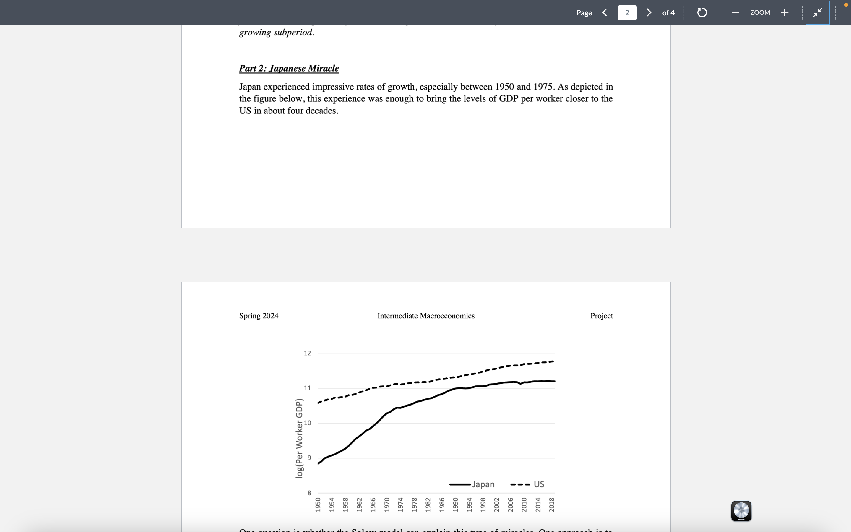
Part 2: Japanese Miracle Japan experienced impressive rates of growth, especially between 1950 and 1975. As depicted in the figure below, this experience was enough to bring the levels of GDP per worker closer to the US in about four decades.
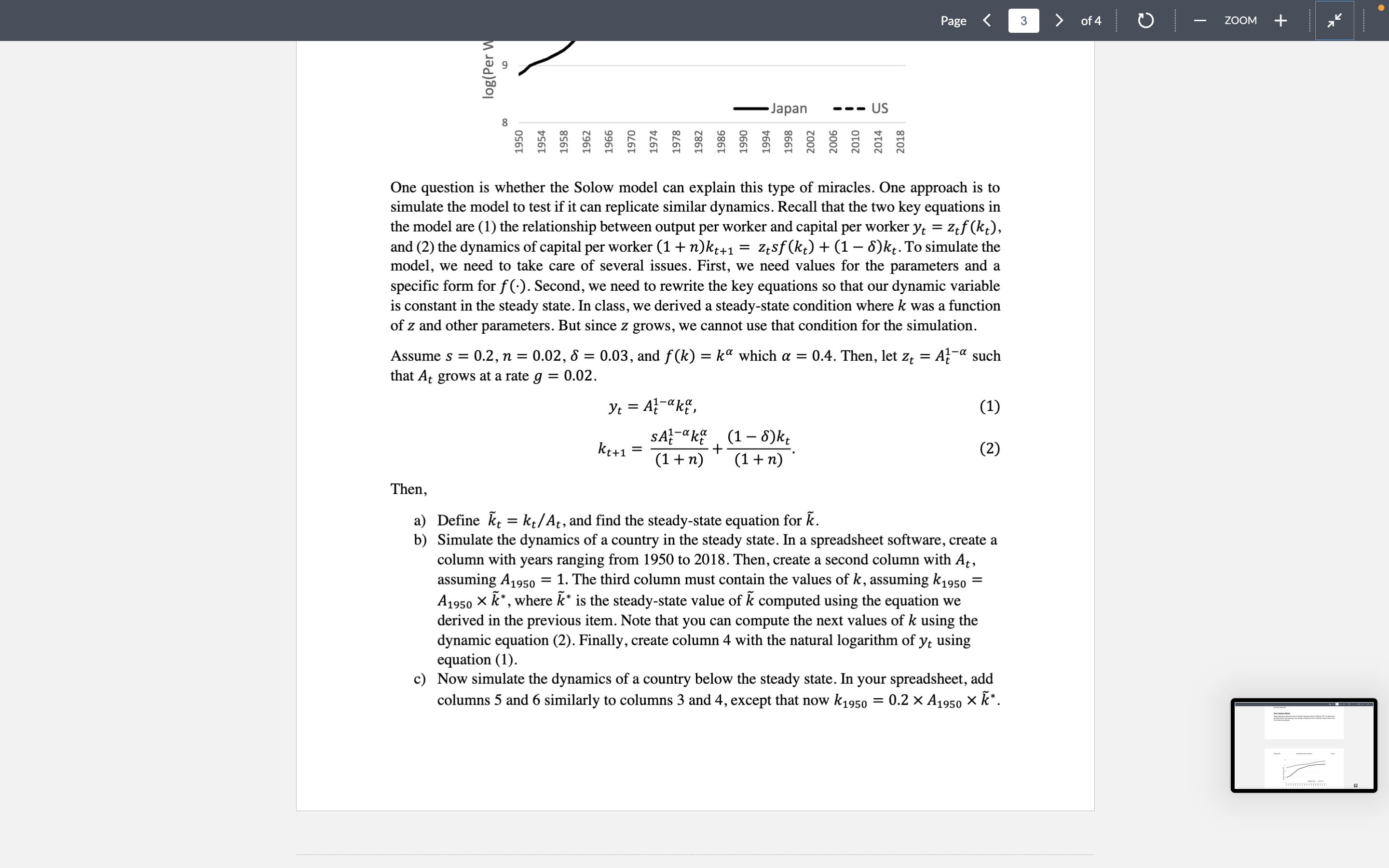
One question is whether the Solow model can explain this type of miracles. One approach is to simulate the model to test if it can replicate similar dynamics. Recall that the two key equations in the model are (1) the relationship between output per worker and capital per worker ?? = ???(??), and (2) the dynamics of capital per worker (1 + ?)??+1 = ????(??) + (1 ? ?)??. To simulate the model, we need to take care of several issues. First, we need values for the parameters and a specific form for ?(?). Second, we need to rewrite the key equations so that our dynamic variable is constant in the steady state. In class, we derived a steady-state condition where ? was a function of ? and other parameters. But since ? grows, we cannot use that condition for the simulation. Assume ? = 0.2, ? = 0.02, ? = 0.03, and ?(?) = ?? which ? = 0.4. Then, let ?? = ?? 1?? such that ?? grows at a rate ? = 0.02. ?? = ?? 1???? ?, (1) ??+1 = ??? 1???? ? (1 + ?) + (1 ? ?)?? (1 + ?) . (2) Then,
a) Define ??? = ?? ??? , and find the steady-state equation for ?? .
b) Simulate the dynamics of a country in the steady state. In a spreadsheet software, make a column with years ranging from 1950 to 2018. Then, create a second column with ??, assuming ?1950 = 1. The third column must contain the values of ?, assuming ?1950 = ?1950 ?? ?, where ?? ? is the steady-state value of ?? computed using the equation we derived in the previous item. Note that you can compute the next values of ? using the dynamic equation (2). Finally, create column 4 with the natural logarithm of ?? using equation (1).
c) Now simulate the dynamics of a country below the steady state. In your spreadsheet, add columns 5 and 6 similarly to columns 3 and 4, except that now ?1950 = 0.2 ?1950 ?? ?. 8 9 10 11 12 1950 1954 1958 1962 1966 1970 1974 1978 1982 1986 1990 1994 1998 2002 2006 2010 2014 2018 log(Per Worker GDP) Japan US
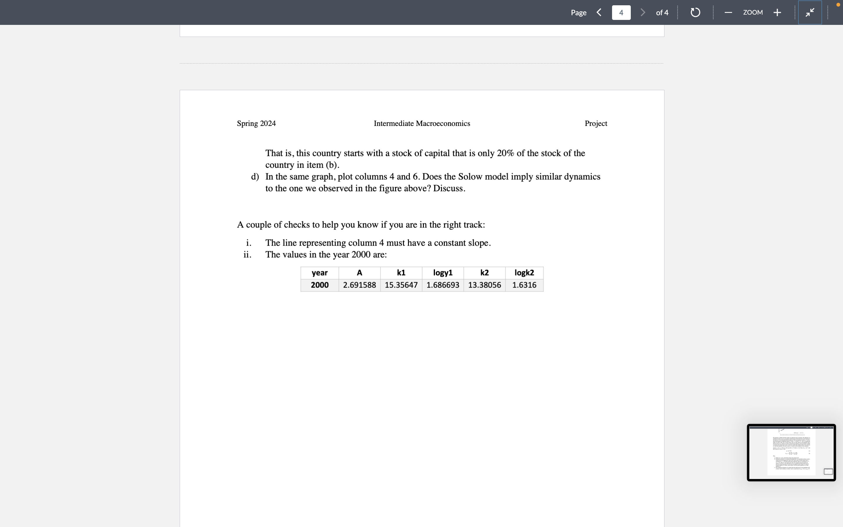
That is, this country starts with a stock of capital that is only 20% of the stock of the country in item (b).
d) In the same graph, plot columns 4 and 6. Does the Solow model imply similar dynamics to the one we observed in the figure above? Discuss.
Show Graphs And Provide Explanations Please.


Step by Step Solution
There are 3 Steps involved in it
Step: 1

Get Instant Access to Expert-Tailored Solutions
See step-by-step solutions with expert insights and AI powered tools for academic success
Step: 2

Step: 3

Ace Your Homework with AI
Get the answers you need in no time with our AI-driven, step-by-step assistance
Get Started


