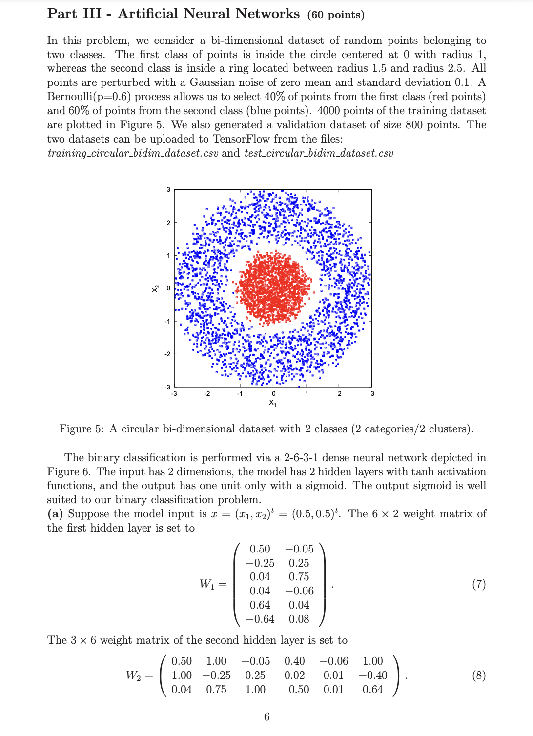
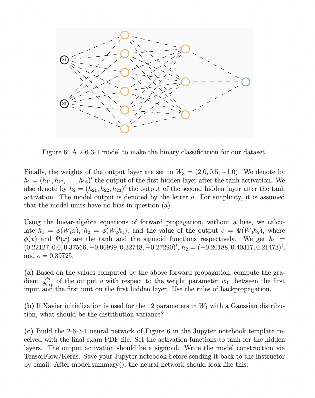
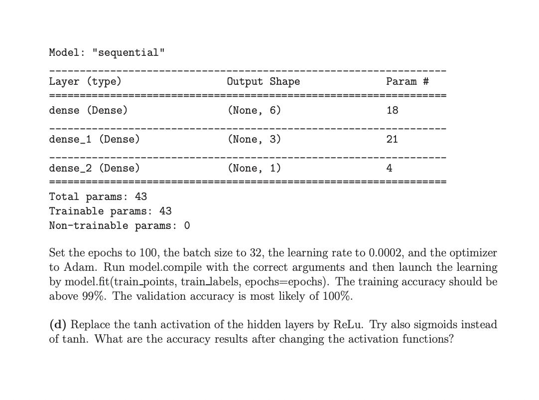
Part III Artificial Neural Networks (60 points) In this problem, we consider a bi-dimensional dataset of random points belonging to two classes. The first class of points is inside the circle centered at 0 with radius 1, whereas the second class is inside a ring located between radius 1.5 and radius 2.5. All points are perturbed with a Gaussian noise of zero mean and standard deviation 0.1. A Bernoulli(p=0.6) process allows us to select 40% of points from the first class (red points) and 60% of points from the second class (blue points). 4000 points of the training dataset are plotted in Figure 5. We also generated a validation dataset of size 800 points. The two datasets can be uploaded to TensorFlow from the files: training_circular_bidim_dataset.csv and test_circular_bidim_dataset.csv 3 2 W = 0 -3 -3 0 X W = Figure 5: A circular bi-dimensional dataset with 2 classes (2 categories/2 clusters). The binary classification is performed via a 2-6-3-1 dense neural network depicted in Figure 6. The input has 2 dimensions, the model has 2 hidden layers with tanh activation functions, and the output has one unit only with a sigmoid. The output sigmoid is well suited to our binary classification problem. (a) Suppose the model input is x = = (x1, x)t = (0.5, 0.5). The 6 x 2 weight matrix of the first hidden layer is set to 0.50 -0.05 -0.25 0.25 0.04 0.75 0.04 -0.06 0.64 0.04 -0.64 0.08 2 The 3 x 6 weight matrix of the second hidden layer is set to 3 6 0.50 1.00 -0.05 0.40 -0.06 1.00 1.00 -0.25 0.25 0.02 0.01 -0.40 0.04 0.75 1.00 -0.50 0.01 0.64 (7) (8) |||||| || | // Figure 6: A 2-6-3-1 model to make the binary classification for our dataset. Finally, the weights of the output layer are set to W3 (2.0, 0.5, -1.0). We denote by h (h11, h12, ..., h16)t the output of the first hidden layer after the tanh activation. We also denote by h (h21, h22, h23) the output of the second hidden layer after the tanh activation. The model output is denoted by the letter o. For simplicity, it is assumed that the model units have no bias in question (a). = = = Using the linear-algebra equations of forward propagation, without a bias, we calcu- late hi (Wx), h (Wh), and the value of the output o (W3h), where (x) and (x) are the tanh and the sigmoid functions respectively. We get h (0.22127, 0.0, 0.37566,-0.00999, 0.32748,-0.27290)t, h = (-0.20188, 0.40317, 0.21473), and o= : 0.39725. = (a) Based on the values computed by the above forward propagation, compute the gra- dient of the output o with respect to the weight parameter w1 between the first input and the first unit on the first hidden layer. Use the rules of backpropagation. dw11 (b) If Xavier initialization is used for the 12 parameters in W with a Gaussian distribu- tion, what should be the distribution variance? (c) Build the 2-6-3-1 neural network of Figure 6 in the Jupyter notebook template re- ceived with the final exam PDF file. Set the activation functions to tanh for the hidden layers. The output activation should be a sigmoid. Write the model construction via TensorFlow/Keras. Save your Jupyter notebook before sending it back to the instructor by email. After model.summary(), the neural network should look like this: Model: "sequential" Layer (type) dense (Dense) dense 1 (Dense) dense 2 (Dense) Total params: 43 Trainable params: 43 Non-trainable params: 0 Output Shape (None, 6) (None, 3) (None, 1) Param # 18 21 4 ====== Set the epochs to 100, the batch size to 32, the learning rate to 0.0002, and the optimizer to Adam. Run model.compile with the correct arguments and then launch the learning by model.fit (train_points, train_labels, epochs epochs). The training accuracy should be above 99%. The validation accuracy is most likely of 100%. (d) Replace the tanh activation of the hidden layers by ReLu. Try also sigmoids instead of tanh. What are the accuracy results after changing the activation functions?