photo is more clear in this pic.. please solve exercise 5.3

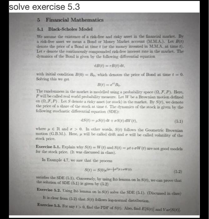
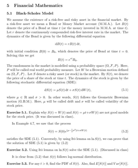
solve exercise 5.3 5 Financial Mathematics 5.1 Black-Scholes Model We assume the existence of a risk-free and risky asset in the financial market. By a risk-free asset we mean a Bond or Money Market account (M.M.A.). Let B(t) denote the price of a Bond at timet (or the money invested in M.M.A. at time t). Letr denote the continuously compounded risk-free interest rate in the market. The dymanics of the Bond is given by the following differential oquation dB(t) = B(t) dt. with initial condition B(O) = Bo, which denotes the price of Bond at time t = 0. Solving this we get B(t) = 2B The randomness in the market is modelled using a probability space (12.F.P). Here, P will be called real world probability measure. Let W be a Brownian motion defined on (2,F,P). Let S denote a risky asset for stock) in the market. By S(t), we denote the price of a share of the stock at time t. The dynamics of the stock is given by the following stochastic differential equation (SDE): 4S(t) = S(t) dt+oS(t)dWt). (5.1) where # E R and a > 0. In other words, s(t) follows the Geometrie Brownian motion (G.B.M.). Here, will be called drift and a will be called volatility of the stock price. Exercise 5.1. Explain why S(t) =Wt) and S(t) = ut+oW (t) are not good models for the stock price. (It was discussed in class). In Example 4.7, we saw that the process s(t) = S(0)elefonown (5.2) satisfies the SDE (5.1). Conversely, by using Ito lemma on in S(t), we can prove that the solution of SDE (5.1) is given by (5.2) Exercise 5.2. Using Iu lemma on In S(t) solve the SDE (5.1). (Discussed in class) It is clear froen (5.2) thuat S(t) follows log-namal distribution Exercise 5.3. For anyt> . find the PDF of S(t). Also, find E[S(t) and Var($(t). 5 Financial Mathematics 5.1 Black-Scholes Model We assume the existence of a risk-free and risky asset in the financial market. By a risk-free asset we mean a Bond or Money Market account (M.M.A.). Let B(t) denote the price of a Bond at time t (or the money invested in M.M.A. at time t). Letr denote the continuously compounded risk-free interest rate in the market. The dymanics of the Bond is given by the following differential equation dB(t) =rB(t) dt, with initial condition B(0) = Bo, which denotes the price of Bond at time t = 0. Solving this we get B(t) = e" B. The randomness in the market is modelled using a probability space (2, F,P). Here, P will be called real world probability measure. Let W be a Brownian motion defined on (22. F,P). Let S denote a risky asset (or stock) in the market. By S(t), we denote the price of a share of the stock at time t. The dynamics of the stock is given by the following stochastic differential equation (SDE): dS(t) = $(t) dt+oS(t)dW (t), (5.1) where pe R and a > 0. In other words, S(t) follows the Geometric Brownian motion (G.B.M.). Here, it will be called drift and a will be called volatility of the stock price. Exercise 5.1. Explain why S(t) =W(t) and S(t) = ut +oW(t) are not good models for the stock price. (It was discussed in class). In Example 4.7, we saw that the process S(t) = S(O)(4-43)+6W(6) (5.2) satisfies the SDE (5.1). Conversely, by using Ito lemma on In S(t), we can prove that the solution of SDE (5.1) is given by (5.2) Exercise 5.2. Using Ito lemma on In S(t) solve the SDE (5.1). (Discussed in class) It is clear from (5.2) that S(t) follows log-normal distribution. Exercise 5.3. For any t > 0, find the PDF of S(t). Also, find E[S(t)] and Var[S(t)). solve exercise 5.3 5 Financial Mathematics 5.1 Black-Scholes Model We assume the existence of a risk-free and risky asset in the financial market. By a risk-free asset we mean a Bond or Money Market account (M.M.A.). Let B(t) denote the price of a Bond at timet (or the money invested in M.M.A. at time t). Letr denote the continuously compounded risk-free interest rate in the market. The dymanics of the Bond is given by the following differential oquation dB(t) = B(t) dt. with initial condition B(O) = Bo, which denotes the price of Bond at time t = 0. Solving this we get B(t) = 2B The randomness in the market is modelled using a probability space (12.F.P). Here, P will be called real world probability measure. Let W be a Brownian motion defined on (2,F,P). Let S denote a risky asset for stock) in the market. By S(t), we denote the price of a share of the stock at time t. The dynamics of the stock is given by the following stochastic differential equation (SDE): 4S(t) = S(t) dt+oS(t)dWt). (5.1) where # E R and a > 0. In other words, s(t) follows the Geometrie Brownian motion (G.B.M.). Here, will be called drift and a will be called volatility of the stock price. Exercise 5.1. Explain why S(t) =Wt) and S(t) = ut+oW (t) are not good models for the stock price. (It was discussed in class). In Example 4.7, we saw that the process s(t) = S(0)elefonown (5.2) satisfies the SDE (5.1). Conversely, by using Ito lemma on in S(t), we can prove that the solution of SDE (5.1) is given by (5.2) Exercise 5.2. Using Iu lemma on In S(t) solve the SDE (5.1). (Discussed in class) It is clear froen (5.2) thuat S(t) follows log-namal distribution Exercise 5.3. For anyt> . find the PDF of S(t). Also, find E[S(t) and Var($(t). 5 Financial Mathematics 5.1 Black-Scholes Model We assume the existence of a risk-free and risky asset in the financial market. By a risk-free asset we mean a Bond or Money Market account (M.M.A.). Let B(t) denote the price of a Bond at time t (or the money invested in M.M.A. at time t). Letr denote the continuously compounded risk-free interest rate in the market. The dymanics of the Bond is given by the following differential equation dB(t) =rB(t) dt, with initial condition B(0) = Bo, which denotes the price of Bond at time t = 0. Solving this we get B(t) = e" B. The randomness in the market is modelled using a probability space (2, F,P). Here, P will be called real world probability measure. Let W be a Brownian motion defined on (22. F,P). Let S denote a risky asset (or stock) in the market. By S(t), we denote the price of a share of the stock at time t. The dynamics of the stock is given by the following stochastic differential equation (SDE): dS(t) = $(t) dt+oS(t)dW (t), (5.1) where pe R and a > 0. In other words, S(t) follows the Geometric Brownian motion (G.B.M.). Here, it will be called drift and a will be called volatility of the stock price. Exercise 5.1. Explain why S(t) =W(t) and S(t) = ut +oW(t) are not good models for the stock price. (It was discussed in class). In Example 4.7, we saw that the process S(t) = S(O)(4-43)+6W(6) (5.2) satisfies the SDE (5.1). Conversely, by using Ito lemma on In S(t), we can prove that the solution of SDE (5.1) is given by (5.2) Exercise 5.2. Using Ito lemma on In S(t) solve the SDE (5.1). (Discussed in class) It is clear from (5.2) that S(t) follows log-normal distribution. Exercise 5.3. For any t > 0, find the PDF of S(t). Also, find E[S(t)] and Var[S(t))