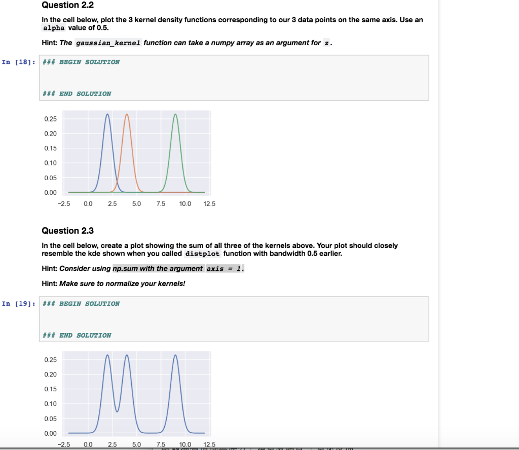
please answer 2.2 and 2.3

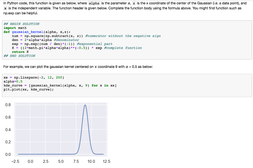
In Python code, this function is given as below, where alpha is the parameter , z is the x coordinate of the center of the Gaussian (i.e. a data point), and x is the independent variable. The function header is given below. Complete the function body using the formula above. You might find function such as np.exp can be helpful ## BEGIN SOLUTION import math def gaussian_kernel (alpha, x,z): num- np. square (np.subtract(x, z)) numerator without the negative sign den 2-alpha-alpha #denominator exp = np.exp ((num / den)" (-1)) #exponential part K = ((2-math .pi-alpha-alpha) **(-0.5)) * exp fcomplete function return K ## END SOLUTION For example, we can plot the gaussian kernel centered on x coordinate 9 with = 0.5 as below: xs -np.linspace (-2, 12, 200) alpha-0.5 kde-curve = [gaussian-kernel ( alpha, x, 9) for x in xs] plt.plot(xs, kde_curve) 0.8 0.6 0.4 0.2 0.0 2.5 0.0 25 5.0 7.50.0 12.5 Question 2.2 In the cell below, plot the 3 kernel density functions corresponding to our 3 data points on the same axis. Use an alpha value of 0.5. Hint: The gaussian kernel function can take a numpy array as an argument for z In [18]: ### BEGIN SOLUTION ### END SOLUTION 0.25 0.20 0.15 0.10 0.05 0.00 -2.5 0.0 25 5.0 7.5 10.0 12.5 Question 2.3 In the cell below, create a plot showing the sum of all three of the kernels above. Your plot should closely resemble the kde shown when you called distplot function with bandwidth 0.5 earlier. Hint: Consider using np.sum with the argument axis-1. Hint: Make sure to normalize your kernels! In [19]: ### BEGIN SOLUTION ### END SOLUTION 0.25 0.20 0.15 0.10 0.05 0.00 2.5 5.0 7.5 10.0 12.5 In Python code, this function is given as below, where alpha is the parameter , z is the x coordinate of the center of the Gaussian (i.e. a data point), and x is the independent variable. The function header is given below. Complete the function body using the formula above. You might find function such as np.exp can be helpful ## BEGIN SOLUTION import math def gaussian_kernel (alpha, x,z): num- np. square (np.subtract(x, z)) numerator without the negative sign den 2-alpha-alpha #denominator exp = np.exp ((num / den)" (-1)) #exponential part K = ((2-math .pi-alpha-alpha) **(-0.5)) * exp fcomplete function return K ## END SOLUTION For example, we can plot the gaussian kernel centered on x coordinate 9 with = 0.5 as below: xs -np.linspace (-2, 12, 200) alpha-0.5 kde-curve = [gaussian-kernel ( alpha, x, 9) for x in xs] plt.plot(xs, kde_curve) 0.8 0.6 0.4 0.2 0.0 2.5 0.0 25 5.0 7.50.0 12.5 Question 2.2 In the cell below, plot the 3 kernel density functions corresponding to our 3 data points on the same axis. Use an alpha value of 0.5. Hint: The gaussian kernel function can take a numpy array as an argument for z In [18]: ### BEGIN SOLUTION ### END SOLUTION 0.25 0.20 0.15 0.10 0.05 0.00 -2.5 0.0 25 5.0 7.5 10.0 12.5 Question 2.3 In the cell below, create a plot showing the sum of all three of the kernels above. Your plot should closely resemble the kde shown when you called distplot function with bandwidth 0.5 earlier. Hint: Consider using np.sum with the argument axis-1. Hint: Make sure to normalize your kernels! In [19]: ### BEGIN SOLUTION ### END SOLUTION 0.25 0.20 0.15 0.10 0.05 0.00 2.5 5.0 7.5 10.0 12.5