please answer fully. this is my third time posting and i cant make sense of this

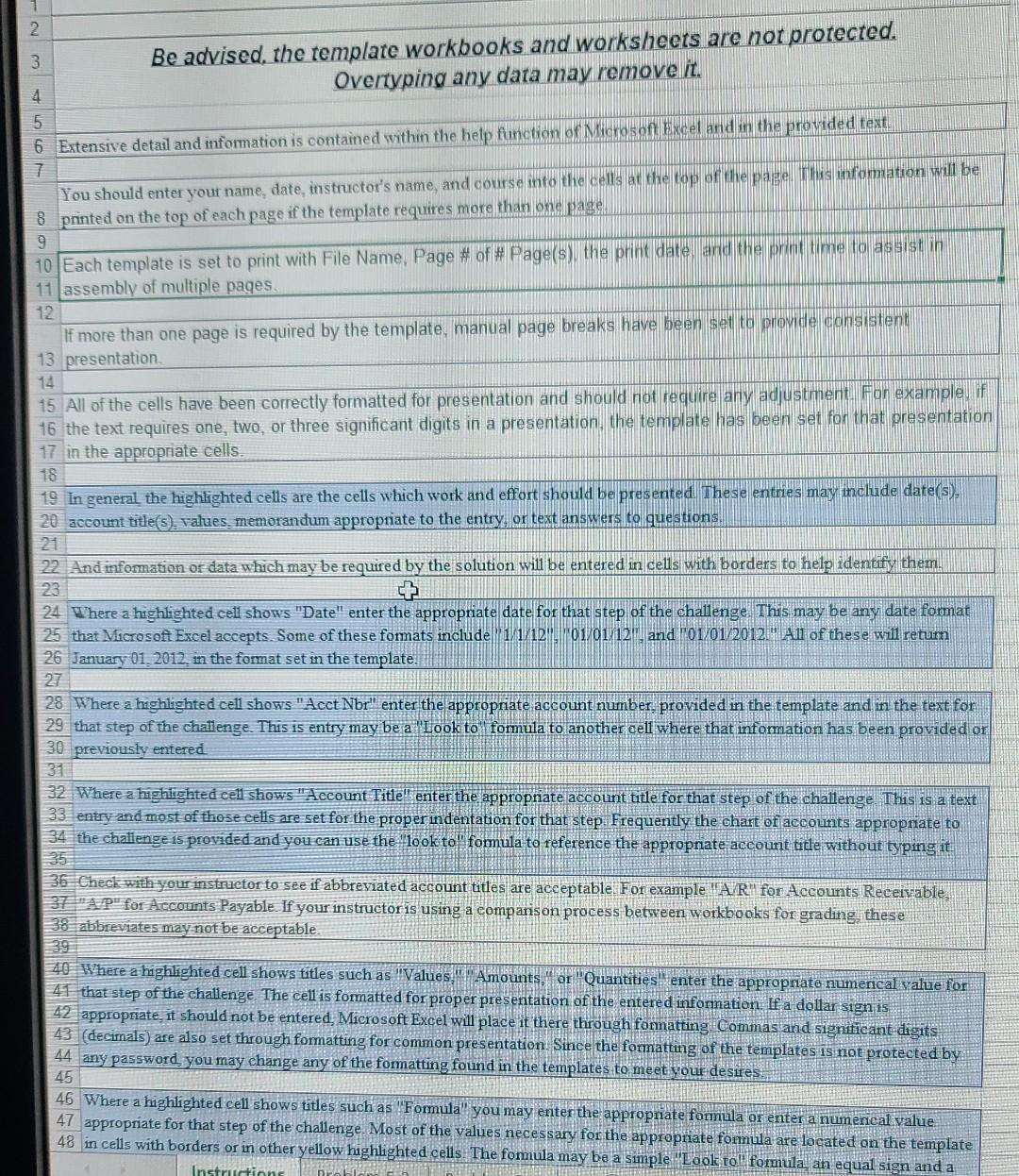
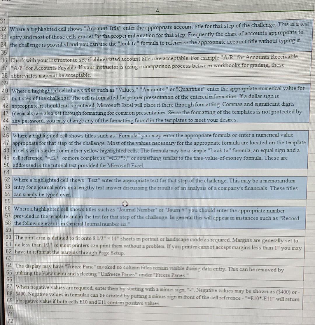
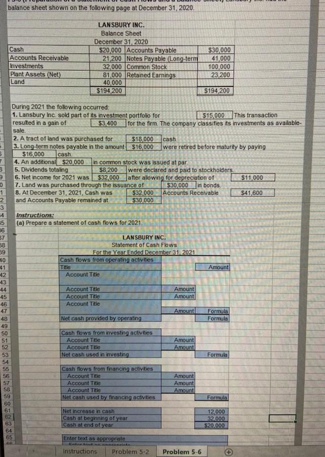
1 2 3 Be advised the template workbooks and worksheets are not protected. Overtyping any data may remove it. W on A 5 6 Extensive detail and information is contained within the help function of Microsoft Excel and in the provided text. You should enter your name, date, instructor's name, and course into the cells at the top of the page. This infomation will be 8 printed on the top of each page if the template requires more than one page, 9 10 Each template is set to print with File Name, Page #of # Page(s) the print date and the print time to assist in 11 assembly of multiple pages. 12 If more than one page is required by the template, manual page breaks have been set to provide consistent 13 presentation 14 15 All of the cells have been correctly formatted for presentation and should not require any adjustment . For example, if 16 the text requires one, two, or three significant digits in a presentation, the template has been set for that presentation 17 in the appropriate cells. 18 19 In general the highlighted cells are the cells which work and effort should be presented. These entries may include date(s). 20 account title(s), values, memorandum appropriate to the entry or text answers to questions 22 And information or data which may be required by the solution will be entered in cells with borders to help identify them. 23 24. Where a highlighted cell shows "Date" enter the appropriate date for that step of the challenge. This may be any date format 25 that Microsoft Excel accepts. Some of these formats include 1/1/12 - 01/01/12", and "01/01/2012." All of these will retum 26 January 01, 2012, in the format set in the template. 27 28 Where a highlighted cell shows "Acct Nbr" enter the appropriate account number, provided in the template and in the text for 29 that step of the challenge. This is entry may be a "'Look to" formula to another cell where that information has been provided or 30 previously entered 31 32 Where a highlighted cell shows "Account Title' enter the appropriate account title for that step of the challenge. This is a text 33 entry and most of these cells are set for the proper indentation for that step. Frequently the chart of accounts appropriate to 34 the challenge is provided and you can use the "look to formula to reference the appropriate account title without typing it. 36 Check with your instructor to see if abbreviated account titles are acceptable. For example "A/R" for Accounts Receivable, 37 "AP" for Accounts Payable. If your instructor is using a companson process between workbooks for grading, these 38 abbreviates may not be acceptable. 40 Where a highlighted cell shows titles such as "Values" "Amounts," or "Quantities! enter the appropriate numerical value for 41 that step of the challenge. The cell is formatted for proper presentation of the entered information. If a dollar sign is 42 appropriate, it should not be entered, Microsoft Excel will place it there through formatting Commas and significant digits 43 (decimals) are also set through formatting for common presentation. Since the formatting of the templates is not protected by 44 any password, you may change any of the formatting found in the templates to meet your desires. 45 46 Where a highlighted cell shows titles such as "Formula" you may enter the appropriate formula or enter a numerical value 47 appropriate for that step of the challenge. Most of the values necessary for the appropriate fomula are located on the template 48 in cells with borders or in other yellow highlighted cells. The formula may be a simple "Look to formula an equal sign and a Instructinne . 31 32 Where a highlighted cell shows "Account Title" enter the appropriate account title for that step of the challenge. This is a text 33 entry and most of those cells are set for the proper indentation for that step. Frequently the chart of accounts appropriate to B4 the challenge is provided and you can use the "look to" formula to reference the appropriate account title without typing it. 35 36 Check with your instructor to see if abbreviated account titles are acceptable. For example "AR" for Accounts Receivable, 37 "AP" for Accounts Payable. If your instructor is using a comparison process between workbooks for grading these 38 abbreviates may not be acceptable. 39 40. Where a hghlighted cell shows tities such as "Values: "Amounts," or "Quantities" enter the appropriate numerical value for 41 that step of the challenge. The cell is formatted for proper presentation of the entered information If a dollar sign is 42 appropriate, it should not be entered Microsoft Excel will place it there through formatting. Commas and significant digits 43 (decimals) are also set through formatting for common presentation. Since the formatting of the templates is not protected by 44 any password, you may change any of the fomatting found in the templates to meet your desires. 45 46. Where a highlighted cell shows titles such as "Formula" you may enter the appropriate formula or enter a numerical value 47 appropriate for that step of the challenge. Most of the values necessary for the appropriate formula are located on the template 48 in cells with borders or in other yellow highlighted cells. The formula may be a simple "Look to" formula, an equal sign and a 49 cell reference. =E27" or more complex as "=E2725," or something similar to the time-value-of-money formula. These are 50 addressed in the tutorial text provided for Microsoft Excel. 51 52 Where a highlighted cell shows "Text" enter the appropriate text for that step of the challenge. This may be a memorandum 53 entry for a joumal entry or a lengthy text answer discussing the results of an analysis of a company's financials. These titles 54 can simply be typed oven 55 56 Where a highlighted cell shows uitles such as "Journal Number" or "Journ you should enter the appropriate number 57 provided in the template and in the text for that step of the challenge In general this will appear in instances such as "Record 58 the following events in General Toumal number 1 59 G0 The print area is defined to fit onto 8 1/2" 11" sheets in portrait or landscape mode as required. Margins are generally set to 61 no less than 12 se most prunters can print them without a problem. If you printer cannot accept margins less than 1" you may 62 have to reformat the margins through Page Setup 63 64 The display may have Freeze Pane" invoked so column titles remain visible during data entry. This can be removed by 65 utilizing the Nessi menu and selecting "Unfreeze Panes" under "Freeze Panes." 66 67 When negative values are required, enter them by starting with a minus sign Negative values may be shown as (5400) or - 68 $400. Negative values in fomulas can be created by putting a minus sign in front of the cell reference - "-E10*-E11" will return 69 A negative value if both cells El0 and Ell contain positive values 170 balance sheet shown on the following page at December 31, 2020, Cash Accounts Receivable Investments Plant Assets (Net) Land LANSBURY INC. Balance Sheet December 31, 2020 $20,000 Accounts Payable 21,200 Notes Payable (Long-term 32,000 Common Stock 81.000 Retained Earnings 40,000 $194,200 $30,000 41,000 100,000 23,200 $194,200 During 2021 the following occurred: 1. Lansbury Inc. sold part of its investment portfolio for S15,000 This transaction resulted in a gain of $3,400 for the firm. The company classifies its investments as available- sale. 2. A tract of land was purchased for $18,000 cash. 3. Long-term notes payable in the amount $16,000 were retired before maturity by paying 5 $16,000 cash. 7 4. An additional $20,000 in common stock was issued at par 3 5. Dividends totaling $8200 were declared and paid to stockholders. 3 6. Net income for 2021 was $32,000 after allowing for depreciation of $11,000 0 7. Land was purchased through the issuance of $30,000 in bonds 1 8. At December 31, 2021, Cash was $32,000 Accounts Receivable $41,600 2 and Accounts Payable remained at $30,000 3 -4 Instructions: 15 (a) Prepare a statement of cash flows for 2021 56 37 LANSBURY INC. 38 Statement of Cash Flows 39 For the Year Ended December 31, 2021 40 Cash flows from operating activities 41 Title Amount 42 Account Title 43 44 Account Title Amount 45 Account Title Amount 46 Account Title Amount Formula 48 Net cash provided by operating Formula 49 SO Cash flows from investing activities 51 Account Title Amount 52 Account Title Amount 53 Net cash used in investing Formula 54 55 Cash flows from financing activities 56 Account Title Amount 57 Account Title Amount 58 Account Title Amount 59 Net cash used by financing activities Formula 60 61 Net increase in cash 12.000 62 Cash at beginning of year 32 000 83 Cash at end of year $20.000 64 65 Enter text as appropriate Instructions Problem 5-2 Problem 5-6 47