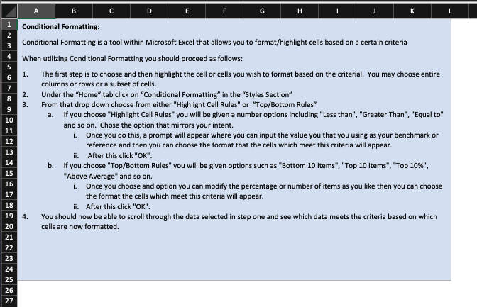
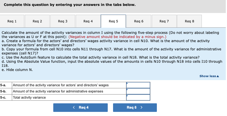
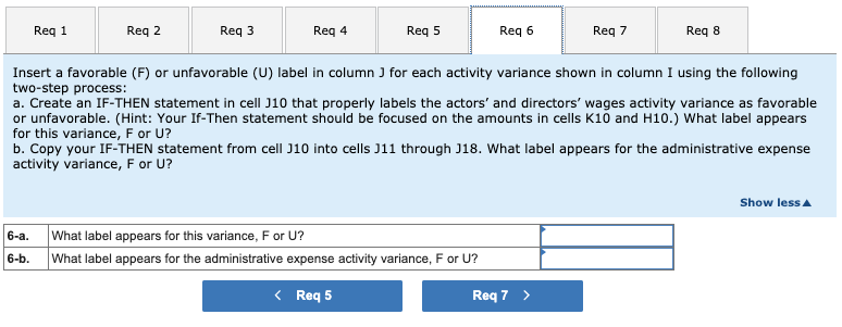
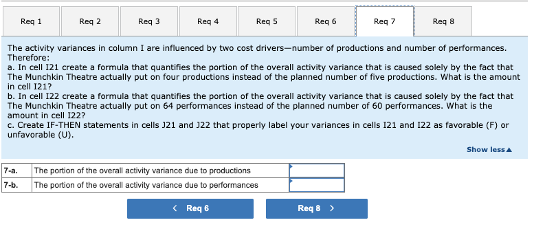
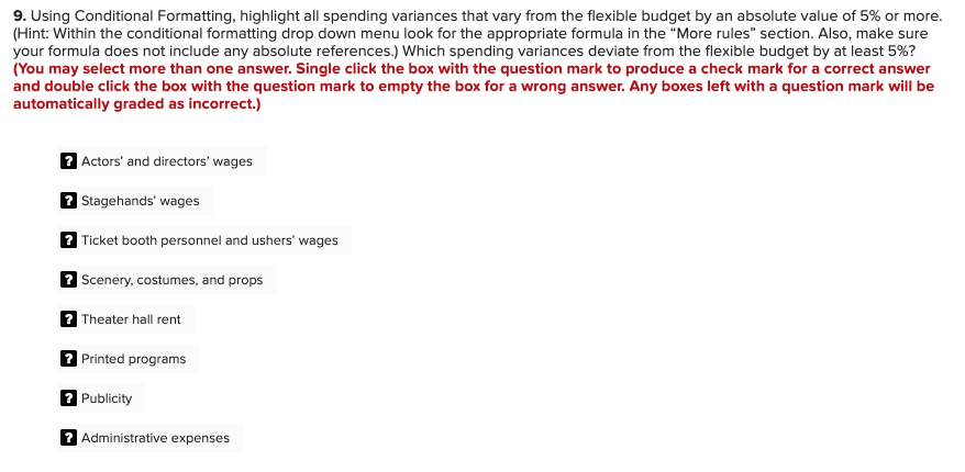
please answer questions Req5-9

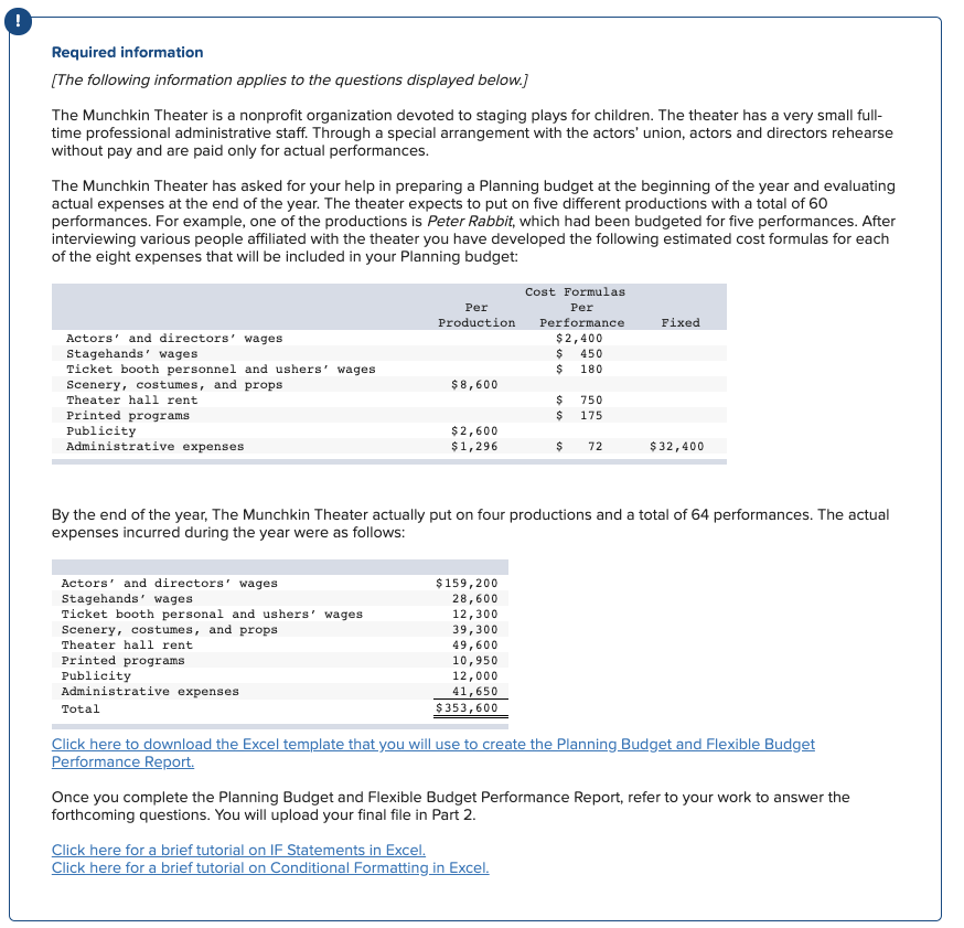
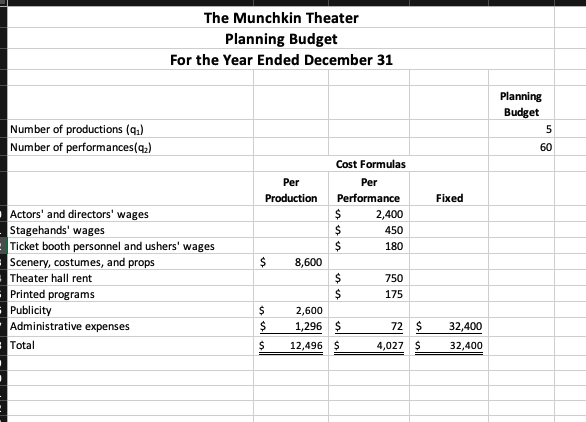
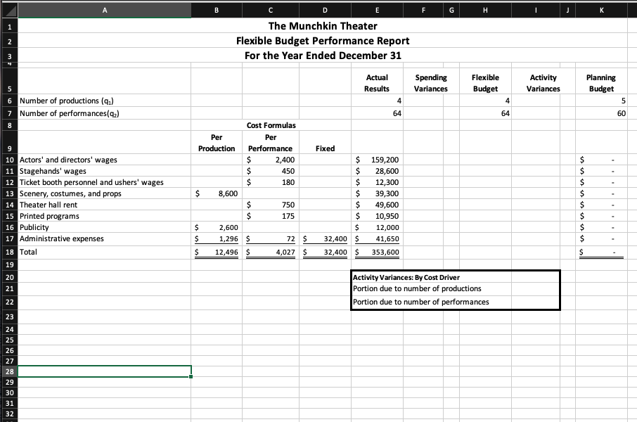
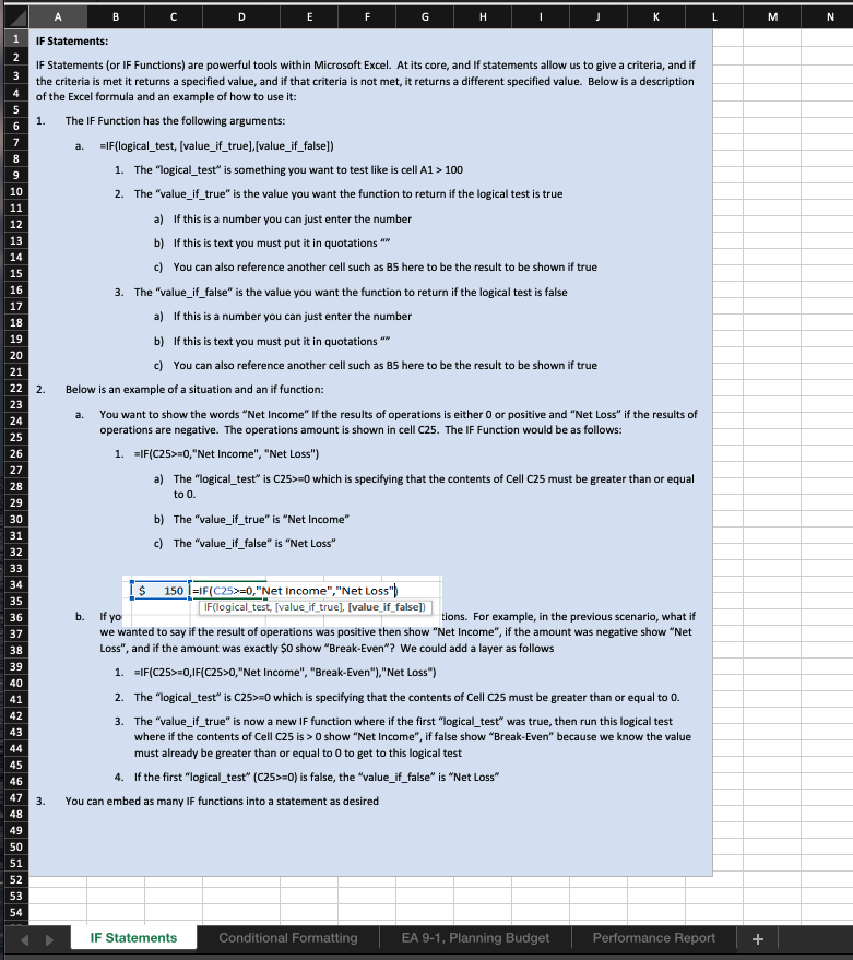
Required information (The following information applies to the questions displayed below.) The Munchkin Theater is a nonprofit organization devoted to staging plays for children. The theater has a very small full- time professional administrative staff. Through a special arrangement with the actors' union, actors and directors rehearse without pay and are paid only for actual performances. The Munchkin Theater has asked for your help in preparing a Planning budget at the beginning of the year and evaluating actual expenses at the end of the year. The theater expects to put on five different productions with a total of 60 performances. For example, one of the productions is Peter Rabbit, which had been budgeted for five performances. After interviewing various people affiliated with the theater you have developed the following estimated cost formulas for each of the eight expenses that will be included in your Planning budget: Per Production Cost Formulas Per Performance $2,400 $ 450 $ 180 Fixed $ 8,600 Actors' and directors' wages Stagehands' wages Ticket booth personnel and ushers' wages Scenery, costumes, and props Theater hall rent Printed programs Publicity Administrative expenses $ $ 750 175 $2,600 $1,296 $ 72 $32,400 By the end of the year, The Munchkin Theater actually put on four productions and a total of 64 performances. The actual expenses incurred during the year were as follows: Actors' and directors' wages Stagehands' wages Ticket booth personal and ushers' wages Scenery, costumes, and props Theater hall rent Printed programs Publicity Administrative expenses Total $159,200 28,600 12,300 39,300 49,600 10,950 12,000 41,650 $ 353,600 Click here to download the Excel template that you will use to create the Planning Budget and Flexible Budget Performance Report Once you complete the Planning Budget and Flexible Budget Performance Report, refer to your work to answer the forthcoming questions. You will upload your final file in Part 2. Click here for a brief tutorial on IF Statements in Excel. Click here for a brief tutorial on Conditional Formatting in Excel. The Munchkin Theater Planning Budget For the Year Ended December 31 Number of productions (9.) Number of performances(42) Planning Budget 5 60 Per Production Fixed Cost Formulas Per Performance $ 2,400 $ 450 180 $ $ 8,600 Actors' and directors' wages Stagehands' wages Ticket booth personnel and ushers' wages Scenery, costumes, and props Theater hall rent Printed programs Publicity Administrative expenses Total 750 175 $ $ $ 2,600 1,296 $ 12,496 $ 72 $ 32,400 32,400 4,027 $ A B D E F H J 1 2 The Munchkin Theater Flexible Budget Performance Report For the Year Ended December 31 3 Actual Results Spending Variances Activity Variances Planning Budget Flexible Budget 4 64 4 5 6 Number of productions (9) 7 Number of performances(92) 8 5 64 60 Per Production Cost Formulas Per Performance $ 2,400 450 180 $ $ 8,600 $ 9 10 Actors' and directors' wages 11 Stagehands' wages 12 Ticket booth personnel and ushers' wages 13 Scenery, costumes, and props 14 Theater hall rent 15 Printed programs 16 Publicity 17 Administrative expenses 18 Total 19 20 21 750 175 Fixed $ 159,200 $ 28,600 $ 12,300 $ 39,300 $ 49,600 $ 10,950 $ 12,000 32,400 $ 41,650 32,400 $ 353,600 $ $ $ $ $ 2,600 1,296 $ 12,496 $ 72 $ $ 4,027 $ $ Activity Variances: By Cost Driver Portion due to number of productions Portion due to number of performances 22 23 24 25 26 27 28 29 30 31 32 D J K L M N IF Statements: 1 2 3 4 5 6 7 1. 8 9 10 11 12 13 14 15 16 17 18 19 20 21 22 23 24 25 26 IF Statements (or IF Functions) are powerful tools within Microsoft Excel. At its core, and if statements allow us to give a criteria, and if the criteria is met it returns a specified value, and if that criteria is not met, it returns a different specified value. Below is a description of the Excel formula and an example of how to use it: The IF Function has the following arguments: a =IF(logical_test, [value_if_true) [value_if_false]) 1. The "logical_test" is something you want to test like is cell A1 > 100 2. The "value_if_true" is the value you want the function to return if the logical test is true a) If this is a number you can just enter the number b) If this is text you must put it in quotations *** c) You can also reference another cell such as BS here to be the result to be shown if true 3. The "value_if_false" is the value you want the function to return if the logical test is false a) If this is a number you can just enter the number b) If this is text you must put it in quotations * c) You can also reference another cell such as B5 here to be the result to be shown if true Below is an example of a situation and an if function: You want to show the words Net Income" If the results of operations is either or positive and "Net Loss" if the results of operations are negative. The operations amount is shown in cell C25. The IF Function would be as follows: 1. =IF(C25>=0, "Net Income", "Net Loss") a) The "logical_test" is C25>=0 which is specifying that the contents of Cell C25 must be greater than or equal 2. a. 27 to O. b) The "value_if_true" is Net Income" c) The "value_if_false" is Net Loss" 28 29 30 31 32 33 34 35 36 37 38 39 40 41 42 43 44 45 46 47 48 49 50 51 52 53 54 150 1 =1F(C25>=0,"Net Income", "Net Loss") IF(logical test, [value_jf true) [value If_false] tions. For example, in the previous scenario, what if b. If yo we wanted to say if the result of operations was positive then show "Net Income", if the amount was negative show "Net Loss", and if the amount was exactly $0 show "Break-Even"? We could add a layer as follows 1. =IF(C25>=0,1F(C25>0, "Net Income", "Break-Even"), "Net Loss") 2. The "logical_test" is c25>=0 which is specifying that the contents of Cell C25 must be greater than or equal to 0. 3. The "value_if_true" is now a new IF function where if the first "logical_test" was true, then run this logical test where if the contents of Cell C25 is > O show "Net Income", if false show "Break-Even" because we know the value must already be greater than or equal to 0 to get to this logical test 4. If the first "logical_test" (C25>=O) is false, the "value_if_false" is Net Loss" You can embed as many IF functions into a statement as desired 3. IF Statements Conditional Formatting EA 9-1, Planning Budget Performance Report + B C D G H I J K L 1. 2. 3. 1 2 3 4 5 6 7 8 9 10 11 12 13 14 15 16 17 18 19 20 21 22 23 24 25 26 27 Conditional Formatting: Conditional Formatting is a tool within Microsoft Excel that allows you to format/highlight cells based on a certain criteria When utilizing Conditional Formatting you should proceed as follows: The first step is to choose and then highlight the cell or cells you wish to format based on the criterial. You may choose entire columns or rows or a subset of cells. Under the "Home" tab click on "Conditional Formatting" in the "Styles Section" From that drop down choose from either "Highlight Cell Rules" or "Top/Bottom Rules" a. If you choose "Highlight Cell Rules" you will be given a number options including "Less than", "Greater Than", "Equal to" and so on. Chose the option that mirrors your intent. i. Once you do this, a prompt will appear where you can input the value you that you using as your benchmark or reference and then you can choose the format that the cells which meet this criteria will appear. ii. After this click "OK". if you choose "Top/Bottom Rules" you will be given options such as "Bottom 10 Items", "Top 10 Items", "Top 10%", "Above Average" and so on. i. Once you choose and option you can modify the percentage or number of items as you like then you can choose the format the cells which meet this criteria will appear. ii. After this click "OK". You should now be able to scroll through the data selected in step one and see which data meets the criteria based on which cells are now formatted. b. Complete this question by entering your answers in the tabs below. Reg 1 Req 2 Req3 Reg 4 Req 5 Req 6 Reg 7 Req 8 Calculate the amount of the activity variances in column I using the following five-step process (Do not worry about labeling the variances as U or F at this point): (Negative amount should be indicated by a minus sign.) a. Create a formula for the actors' and directors' wages activity variance in cell N10. What is the amount of the activity variance for actors' and directors' wages? b. Copy your formula from cell N10 into cells N11 through N17. What is the amount of the activity variance for administrative expenses (cell N17)? c. Use the AutoSum feature to calculate the total activity variance in cell N18. What is the total activity variance? d. Using the Absolute Value function, input the absolute values of the amounts in cells N10 through Nis into cells 110 through 118. e. Hide column N. Show less 5-a. Amount of the activity variance for actors' and directors' wages 5-b. Amount of the activity variance for administrative expenses 5-c. Total activity variance Reg 1 Reg 2 Req 3 Req 4 Req 5 Reg 6 Reg 7 Reg 8 Insert a favorable (F) or unfavorable (U) label in column ) for each activity variance shown in column I using the following two-step process: a. Create an IF-THEN statement in cell J10 that properly labels the actors' and directors' wages activity variance as favorable or unfavorable. (Hint: Your If-Then statement should be focused on the amounts in cells K10 and H10.) What label appears for this variance, F or U? b. Copy your IF-THEN statement from cell J10 into cells J11 through J18. What label appears for the administrative expense activity variance, F or U? Show less 6-a. What label appears for this variance, For U? What label appears for the administrative expense activity variance, F or U? 6-b. Reg 1 Req 2 Req3 Req 4 Req 5 Req6 Req 7 Req 8 The activity variances in column I are influenced by two cost drivers-number of productions and number of performances. Therefore: a. In cell 121 create a formula that quantifies the portion of the overall activity variance that is caused solely by the fact that The Munchkin Theatre actually put on four productions instead of the planned number of five productions. What is the amount in cell 1212 b. In cell 122 create a formula that quantifies the portion of the overall activity variance that is caused solely by the fact that The Munchkin Theatre actually put on 64 performances instead of the planned number of 60 performances. What is the amount in cell 122? c. Create IF-THEN statements in cells 221 and 122 that properly label your variances in cells 121 and 122 as favorable (F) or unfavorable (U). Show less 7-a. The portion of the overall activity variance due to productions The portion of the overall activity variance due to performances 7-b. Reg 1 Reg 2 Req 3 Reg 4 Req 5 Req6 Reg 7 Req 8 Using Conditional Formatting, highlight all spending variances that varied by an absolute value of $1,000 or more. How many of the spending variances are highlighted? Number of spending variances highlighted 100 2. The "value_if_true" is the value you want the function to return if the logical test is true a) If this is a number you can just enter the number b) If this is text you must put it in quotations *** c) You can also reference another cell such as BS here to be the result to be shown if true 3. The "value_if_false" is the value you want the function to return if the logical test is false a) If this is a number you can just enter the number b) If this is text you must put it in quotations * c) You can also reference another cell such as B5 here to be the result to be shown if true Below is an example of a situation and an if function: You want to show the words Net Income" If the results of operations is either or positive and "Net Loss" if the results of operations are negative. The operations amount is shown in cell C25. The IF Function would be as follows: 1. =IF(C25>=0, "Net Income", "Net Loss") a) The "logical_test" is C25>=0 which is specifying that the contents of Cell C25 must be greater than or equal 2. a. 27 to O. b) The "value_if_true" is Net Income" c) The "value_if_false" is Net Loss" 28 29 30 31 32 33 34 35 36 37 38 39 40 41 42 43 44 45 46 47 48 49 50 51 52 53 54 150 1 =1F(C25>=0,"Net Income", "Net Loss") IF(logical test, [value_jf true) [value If_false] tions. For example, in the previous scenario, what if b. If yo we wanted to say if the result of operations was positive then show "Net Income", if the amount was negative show "Net Loss", and if the amount was exactly $0 show "Break-Even"? We could add a layer as follows 1. =IF(C25>=0,1F(C25>0, "Net Income", "Break-Even"), "Net Loss") 2. The "logical_test" is c25>=0 which is specifying that the contents of Cell C25 must be greater than or equal to 0. 3. The "value_if_true" is now a new IF function where if the first "logical_test" was true, then run this logical test where if the contents of Cell C25 is > O show "Net Income", if false show "Break-Even" because we know the value must already be greater than or equal to 0 to get to this logical test 4. If the first "logical_test" (C25>=O) is false, the "value_if_false" is Net Loss" You can embed as many IF functions into a statement as desired 3. IF Statements Conditional Formatting EA 9-1, Planning Budget Performance Report + B C D G H I J K L 1. 2. 3. 1 2 3 4 5 6 7 8 9 10 11 12 13 14 15 16 17 18 19 20 21 22 23 24 25 26 27 Conditional Formatting: Conditional Formatting is a tool within Microsoft Excel that allows you to format/highlight cells based on a certain criteria When utilizing Conditional Formatting you should proceed as follows: The first step is to choose and then highlight the cell or cells you wish to format based on the criterial. You may choose entire columns or rows or a subset of cells. Under the "Home" tab click on "Conditional Formatting" in the "Styles Section" From that drop down choose from either "Highlight Cell Rules" or "Top/Bottom Rules" a. If you choose "Highlight Cell Rules" you will be given a number options including "Less than", "Greater Than", "Equal to" and so on. Chose the option that mirrors your intent. i. Once you do this, a prompt will appear where you can input the value you that you using as your benchmark or reference and then you can choose the format that the cells which meet this criteria will appear. ii. After this click "OK". if you choose "Top/Bottom Rules" you will be given options such as "Bottom 10 Items", "Top 10 Items", "Top 10%", "Above Average" and so on. i. Once you choose and option you can modify the percentage or number of items as you like then you can choose the format the cells which meet this criteria will appear. ii. After this click "OK". You should now be able to scroll through the data selected in step one and see which data meets the criteria based on which cells are now formatted. b. Complete this question by entering your answers in the tabs below. Reg 1 Req 2 Req3 Reg 4 Req 5 Req 6 Reg 7 Req 8 Calculate the amount of the activity variances in column I using the following five-step process (Do not worry about labeling the variances as U or F at this point): (Negative amount should be indicated by a minus sign.) a. Create a formula for the actors' and directors' wages activity variance in cell N10. What is the amount of the activity variance for actors' and directors' wages? b. Copy your formula from cell N10 into cells N11 through N17. What is the amount of the activity variance for administrative expenses (cell N17)? c. Use the AutoSum feature to calculate the total activity variance in cell N18. What is the total activity variance? d. Using the Absolute Value function, input the absolute values of the amounts in cells N10 through Nis into cells 110 through 118. e. Hide column N. Show less 5-a. Amount of the activity variance for actors' and directors' wages 5-b. Amount of the activity variance for administrative expenses 5-c. Total activity variance Reg 1 Reg 2 Req 3 Req 4 Req 5 Reg 6 Reg 7 Reg 8 Insert a favorable (F) or unfavorable (U) label in column ) for each activity variance shown in column I using the following two-step process: a. Create an IF-THEN statement in cell J10 that properly labels the actors' and directors' wages activity variance as favorable or unfavorable. (Hint: Your If-Then statement should be focused on the amounts in cells K10 and H10.) What label appears for this variance, F or U? b. Copy your IF-THEN statement from cell J10 into cells J11 through J18. What label appears for the administrative expense activity variance, F or U? Show less 6-a. What label appears for this variance, For U? What label appears for the administrative expense activity variance, F or U? 6-b. Reg 1 Req 2 Req3 Req 4 Req 5 Req6 Req 7 Req 8 The activity variances in column I are influenced by two cost drivers-number of productions and number of performances. Therefore: a. In cell 121 create a formula that quantifies the portion of the overall activity variance that is caused solely by the fact that The Munchkin Theatre actually put on four productions instead of the planned number of five productions. What is the amount in cell 1212 b. In cell 122 create a formula that quantifies the portion of the overall activity variance that is caused solely by the fact that The Munchkin Theatre actually put on 64 performances instead of the planned number of 60 performances. What is the amount in cell 122? c. Create IF-THEN statements in cells 221 and 122 that properly label your variances in cells 121 and 122 as favorable (F) or unfavorable (U). Show less 7-a. The portion of the overall activity variance due to productions The portion of the overall activity variance due to performances 7-b. Reg 1 Reg 2 Req 3 Reg 4 Req 5 Req6 Reg 7 Req 8 Using Conditional Formatting, highlight all spending variances that varied by an absolute value of $1,000 or more. How many of the spending variances are highlighted? Number of spending variances highlighted