PLEASE ANSWER QUESTIONS WITH FORMULA STEP BY STEP - EXCEL.
excel questions, pls answer questions in excel.
will upvote thanks :)

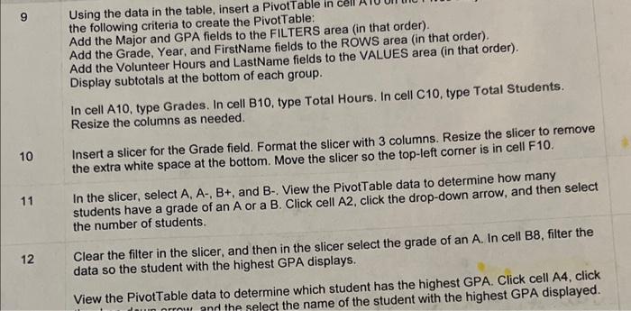
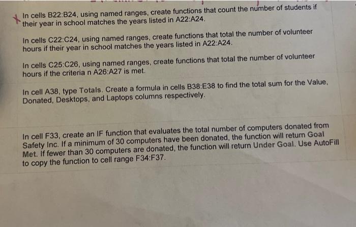
9 Using the data in the table, insert a PivotTable the following criteria to create the PivolTable: Add the Major and GPA fields to the FILTER, Year, and FirstName fields to the ROWS area (in that order). Add the Grade, Year, and FirstName fields to the Hours and LastName fields to the VALUES area (in that order). Add the Voluntay subtotals at the bottom of each group. In cell A10, type Grades. In cell B10, type Total Hours. In cell C10, type Total Students. Resize the columns as needed. 10 Insert a slicer for the Grade field. Format the slicer with 3 columns. Resize the slicer to remove the extra white space at the bottom. Move the slicer so the top-left corner is in cell F10. 11 In the slicer, select A,AB+, and B-. View the PivotTable data to determine how many students have a grade of an A or a B. Click cell A2, click the drop-down arrow, and then select the number of students. 12 Clear the filter in the slicer, and then in the slicer select the grade of an A. In cell B8, filter the data so the student with the highest GPA displays. View the PivotTable data to determine which student has the highest GPA. Click cell A4, click In cells B22:B24, using named ranges, create functions that count the number of students if their year in school matches the years listed in A22:A24. In cells C22:C24, using named ranges, create functions that total the number of volunteer hours if their year in school matches the years listed in A22:A24. In cells C25:C26, using named ranges, create functions that total the number of volunteer hours if the criteria n A26:A27 is met. In cell A38, type Totals. Create a formula in cells B38:E38 to find the total sum for the Value, Donated, Desktops, and Laptops columns respectively. In cell F33, create an IF function that evaluates the total number of computers donated from Safety Inc. If a minimum of 30 computers have been donated, the function will return Goal Met. If fewer than 30 computers are donated, the function will return Under Goal. Use AutoFill to copy the function to cell range F34:F37. 9 Using the data in the table, insert a PivotTable the following criteria to create the PivolTable: Add the Major and GPA fields to the FILTER, Year, and FirstName fields to the ROWS area (in that order). Add the Grade, Year, and FirstName fields to the Hours and LastName fields to the VALUES area (in that order). Add the Voluntay subtotals at the bottom of each group. In cell A10, type Grades. In cell B10, type Total Hours. In cell C10, type Total Students. Resize the columns as needed. 10 Insert a slicer for the Grade field. Format the slicer with 3 columns. Resize the slicer to remove the extra white space at the bottom. Move the slicer so the top-left corner is in cell F10. 11 In the slicer, select A,AB+, and B-. View the PivotTable data to determine how many students have a grade of an A or a B. Click cell A2, click the drop-down arrow, and then select the number of students. 12 Clear the filter in the slicer, and then in the slicer select the grade of an A. In cell B8, filter the data so the student with the highest GPA displays. View the PivotTable data to determine which student has the highest GPA. Click cell A4, click In cells B22:B24, using named ranges, create functions that count the number of students if their year in school matches the years listed in A22:A24. In cells C22:C24, using named ranges, create functions that total the number of volunteer hours if their year in school matches the years listed in A22:A24. In cells C25:C26, using named ranges, create functions that total the number of volunteer hours if the criteria n A26:A27 is met. In cell A38, type Totals. Create a formula in cells B38:E38 to find the total sum for the Value, Donated, Desktops, and Laptops columns respectively. In cell F33, create an IF function that evaluates the total number of computers donated from Safety Inc. If a minimum of 30 computers have been donated, the function will return Goal Met. If fewer than 30 computers are donated, the function will return Under Goal. Use AutoFill to copy the function to cell range F34:F37
