Please answer these questions thanks. I'm confused.

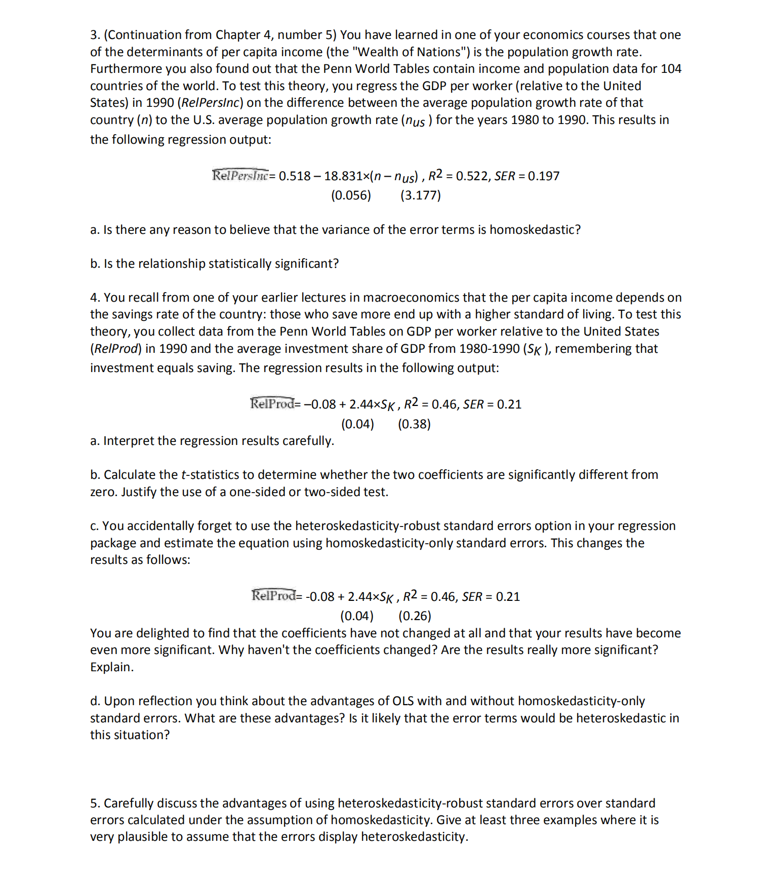
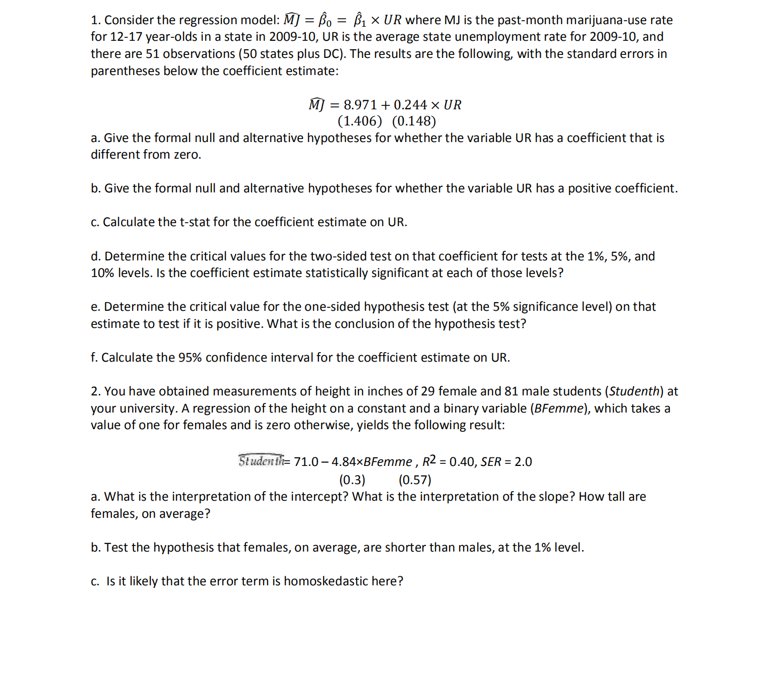
3. [Continuation from Chapter 4, number 5) You have learned in one of your economics courses that one of the determinants of per capita income (the "Wealth of Nations\") is the population growth rate. Furthermore you also found out that the Penn World Tables contain income and population data for 104 countries of the world. To test this theory, you regress the GDP per worker (relative to the United States) in 1990 (RelPersInc) on the difference between the average population growth rate of that country (n) to the U.S. average population growth rate ("us ) for the years 1980 to 1990. This results in the following regression output: fawn\"In = 0.513 18.831x(n nus) , R2 = 0.522, 5.50 = 0.197 (0.055) (3.177) a. Is there any reason to believe that the variance of the error terms is homoskedastic? b. Is the relationship statistically significant? 4. You recall from one of your earlier lectures in macroeconomics that the per capita income depends on the savings rate of the country: those who save more end up with a higher standard of living. To test this theory, you collect data from the Penn World Tables on GDP per worker relative to the United States (RelProd) in 1990 and the average investment share of GDP from 1980-1990 (5K ), remembering that investment equals saving. The regression results in the following output: elPro = 0.08 + 2.44x5K, R2 = 0.45, SER = 0.21 (0.04) (0.38) a. Interpret the regression results carefully. b. Calculate the tstatistics to determine whether the two coefficients are significantly different from zero. Justify the use of a one-sided or two-sided test. c. You accidentally forget to use the heteroskedasticity-robust standard errors option in your regression package and estimate the equation using homoskedasticity-only standard errors. This changes the results as follows: elPruH= -0.03 + 2.44x5K, R2 = 0.46, SER = 0.21 (0.04) (0.26) You are delighted to find that the coefficients have not changed at all and that your results have become even more significant. Why haven't the coefficients changed? Are the results really more significant? Explain. d. Upon reflection you think about the advantages of OLS with and without homoskedasticityonly standard errors. What are these advantages? Is it likely that the error terms would be heteroskedastic in this situation? 5. Carefully discuss the advantages of using heteroskedasticity-robust standard errors over standard errors calculated under the assumption of homoskedasticity. Give at least three examples where it is very plausible to assume that the errors display heteroskedasticity. 1. Consider the regression model: M] = 30 = 31 x UR where MJ is the past-month marijuana-use rate for 12-17 year-olds in a state in 2009-10, UR is the average state unemployment rate for 2009-10, and there are 51 observations (50 states plus DC). The results are the following, with the standard errors in parentheses below the coefficient estimate: M] = 8.971 + 0.244 x UR (1.406) (0.148) a. Give the formal null and alternative hypotheses for whether the variable UR has a coefficient that is different from zero. b. Give the formal null and alternative hypotheses for whether the variable UR has a positive coefficient. c. Calculate the t-stat for the coefficient estimate on UR. d. Determine the critical values for the twosided test on that coefficient for tests at the 1%, 5%, and 10% levels. Is the coefficient estimate statistically significant at each of those levels? e. Determine the critical value for the one-sided hypothesis test (at the 5% significance level) on that estimate to test if it is positive. What is the conclusion of the hypothesis test? f. Calculate the 95% confidence interval for the coefficient estimate on UR. 2. You have obtained measurements of height in inches of 29 female and 81 male students (Studenth) at your university. A regression of the height on a constant and a binary variable (BFemme), which takes a value of one for females and is zero otherwise, yields the following result: E'rudm'r'm 71.0 4.84xBFemme, R2 = 0.40, SER = 2.0 (0.3) (0.57) a. What is the interpretation of the intercept? What is the interpretation of the slope? How tall are females, on average? b. Test the hypothesis that females, on average, are shorter than males, at the 1% level. (3. Is it likely that the error term is homoskedastic here