Please code this, I will give thumbs up!


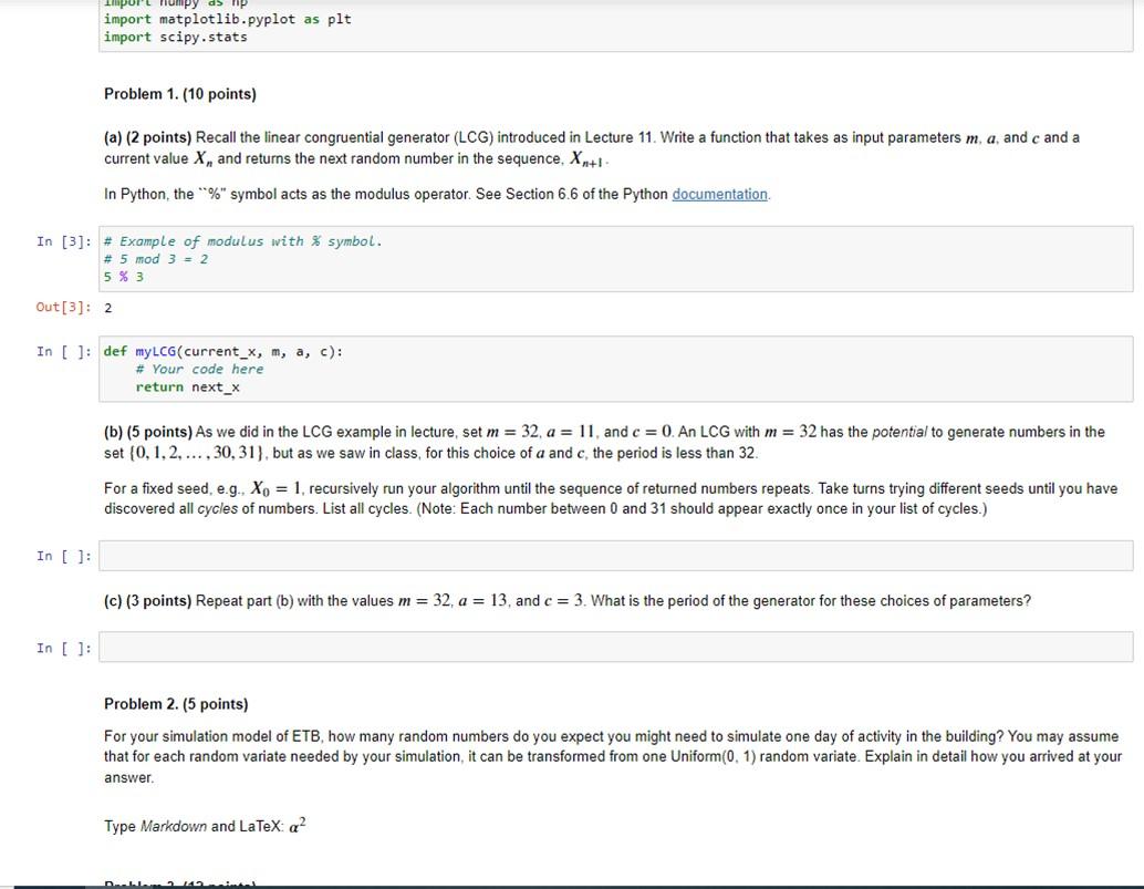
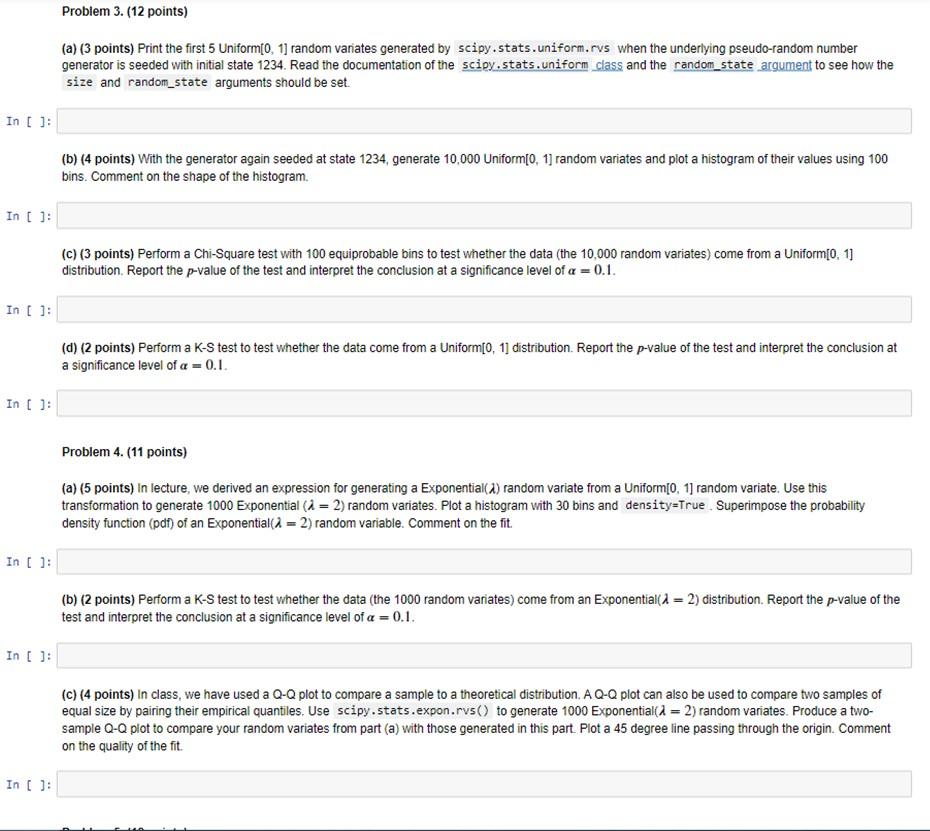
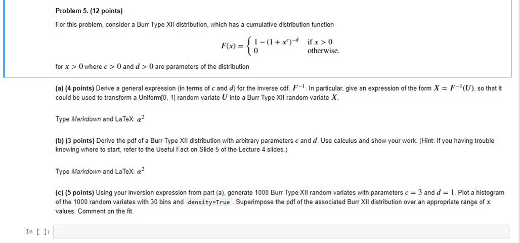
(a) (2 points) Recall the linear congruential generator (LCG) introduced in Lecture 11. Write a function that takes as input parameters m, a, and c and a current value Xn and returns the next random number in the sequence, Xn+1. In Python, the "\%" symbol acts as the modulus operator. See Section 6.6 of the Python \# Example of modulus with % symbol. \# 5 mod 3=2 5%3 :2 def mylcG(current_x, m,a,c) : \# Your code here return next_x (b) (5 points) As we did in the LCG example in lecture, set m=32, a=11, and c=0. An LCG with m=32 has the potential to generate numbers in the set {0,1,2,,30,31}, but as we saw in class, for this choice of a and c, the period is less than 32 . For a fixed seed, e.g., X0=1, recursively run your algorithm until the sequence of returned numbers repeats. Take turns trying different seeds until you have discovered all cycles of numbers. List all cycles. (Note: Each number between 0 and 31 should appear exactly once in your list of cycles.) (c) (3 points) Repeat part (b) with the values m=32,a=13, and c=3. What is the period of the generator for these choices of parameters? Problem 2. (5 points) For your simulation model of ETB, how many random numbers do you expect you might need to simulate one day of activity in the building? You may assume that for each random variate needed by your simulation, it can be transformed from one Uniform (0,1) random variate. Explain in detail how you arrived at your answer. Type Markdown and LaTeX: 2 (a) (3 points) Print the first 5 Uniform [0,1] random variates generated by scipy. stats. uniform. rvs when the underlying pseudo-random number generator is seeded with initial state 1234. Read the documentation of the scipy.stats. uniform class and the random_state argument to see how the size and random_state arguments should be set. (b) (4 points) With the generator again seeded at state 1234 , generate 10,000 Uniform[0, 1] random variates and plot a histogram of their values using 100 bins. Comment on the shape of the histogram. (c) (3 points) Perform a Chi-Square test with 100 equiprobable bins to test whether the data (the 10,000 random variates) come from a Uniform[0, 1] distribution. Report the p-value of the test and interpret the conclusion at a significance level of =0.1. (d) (2 points) Perform a K-S test to test whether the data come from a Uniform [0,1] distribution. Report the p-value of the test and interpret the conclusion at a significance level of =0.1. Problem 4. (11 points) (a) (5 points) In lecture, we derived an expression for generating a Exponential () random variate from a Uniform [0,1] random variate. Use this transformation to generate 1000 Exponential (=2) random variates. Plot a histogram with 30 bins and density=True. Superimpose the probability density function (pdf) of an Exponential (=2) random variable. Comment on the fit. (b) (2 points) Perform a K-S test to test whether the data (the 1000 random variates) come from an Exponential( =2) distribution. Report the p-value of the test and interpret the conclusion at a significance level of =0.1. (c) (4 points) In class, we have used a Q-Q plot to compare a sample to a theoretical distribution. A Q-Q plot can also be used to compare two samples of equal size by pairing their empirical quantiles. Use scipy. stats. expon. rvs() to generate 1000 Exponential (=2) random variates. Produce a twosample Q-Q plot to compare your random variates from part (a) with those generated in this part. Plot a 45 degree line passing through the origin. Comment on the quality of the fit. Problem 5. (12 points) For this problem, consider a Burr Type XII distribution, which has a cumulative distribution function F(x)={1(1+xc)d0ifx>0otherwise for x>0 where c>0 and d>0 are parameters of the distribution (a) (4 points) Derive a general expression (in terms of c and d ) for the inverse cdf, F1. In particular, give an expression of the form X=F1(U), so that it could be used to transform a Uniform [0,1] random variate U into a Burr Type XII random variate X. Type Markdown and LaTeX: 2 (b) (3 points) Derive the pdi of a Burr Type XII distribution with arbitrary parameters c and d. Use calculus and show your work. (Hint: If you having trouble knowing where to start, refer to the Useful Fact on Slide 5 of the Lecture 4 slides.) Type Markdown and LaTeX: 2 (c) (5 points) Using your inversion expression from part (a), generate 1000 Burr Type XII random variates with parameters c=3 and d=1. Plot a histogram of the 1000 random variates with 30 bins and density=True. Superimpose the pdf of the associated Burr XII distribution over an appropriate range of x values. Comment on the fit
