Please complete procedure A.

all the data needed from experiment has been provided you must use the formulas to fill in the missing boxes.

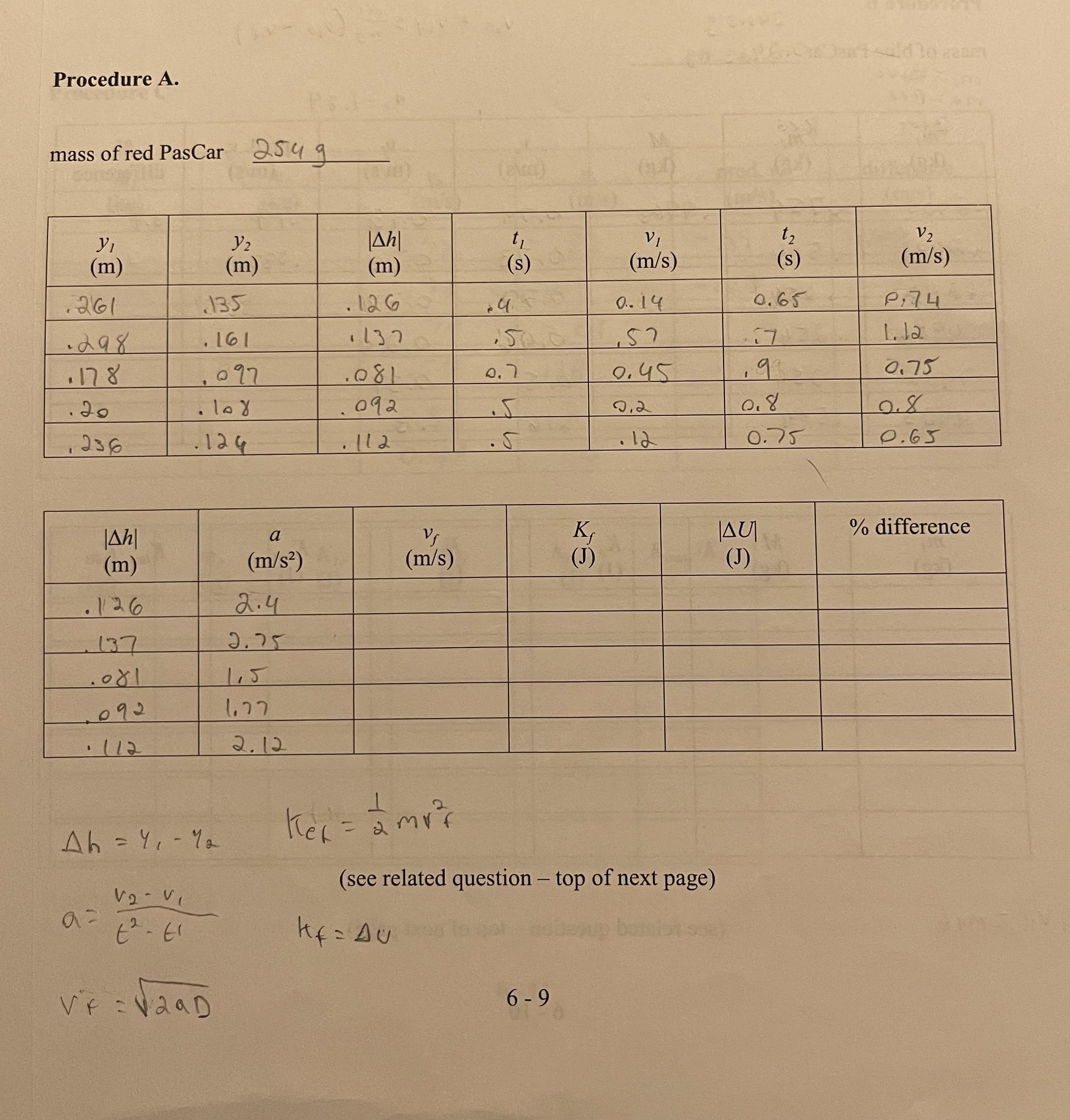
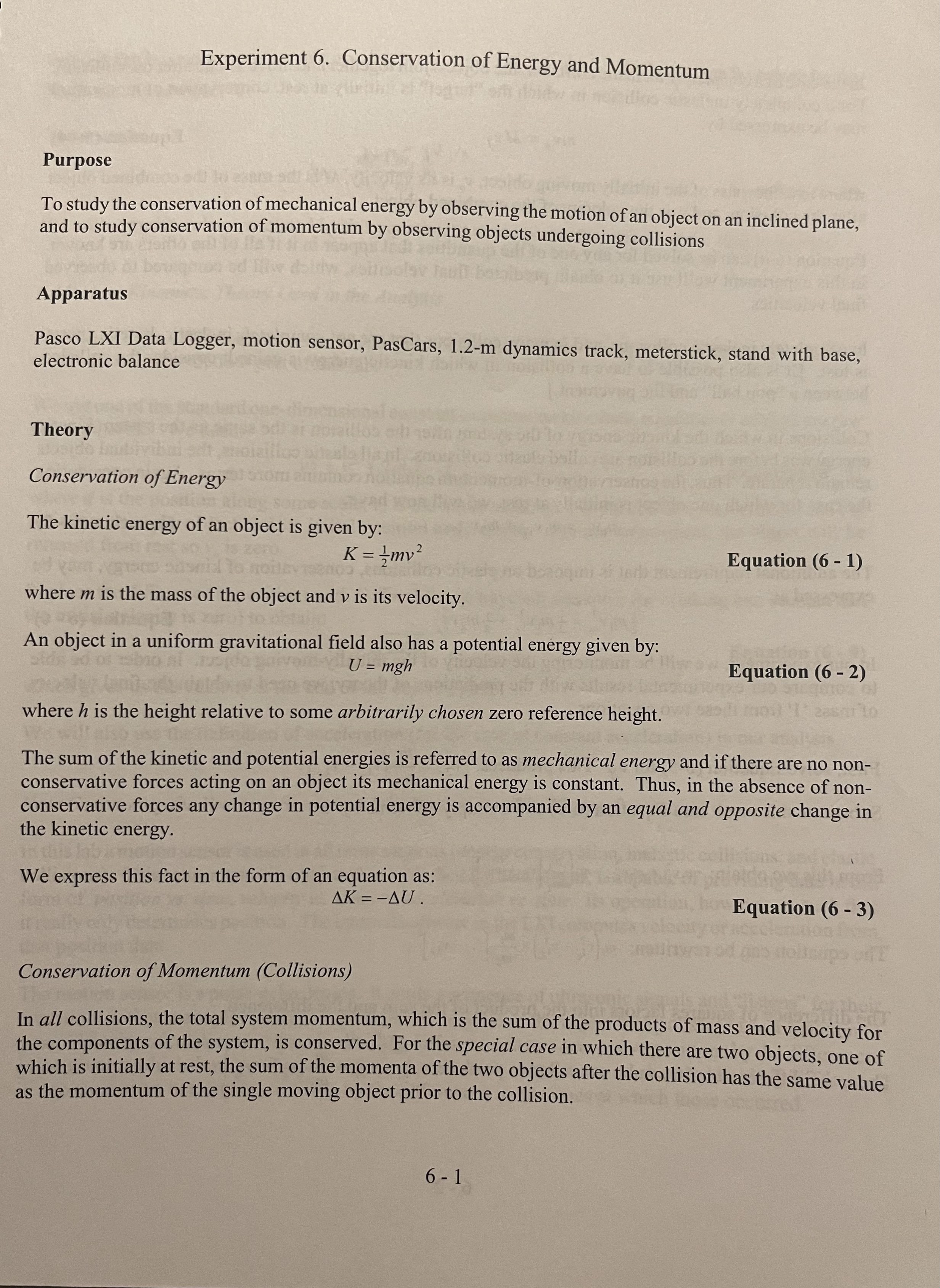
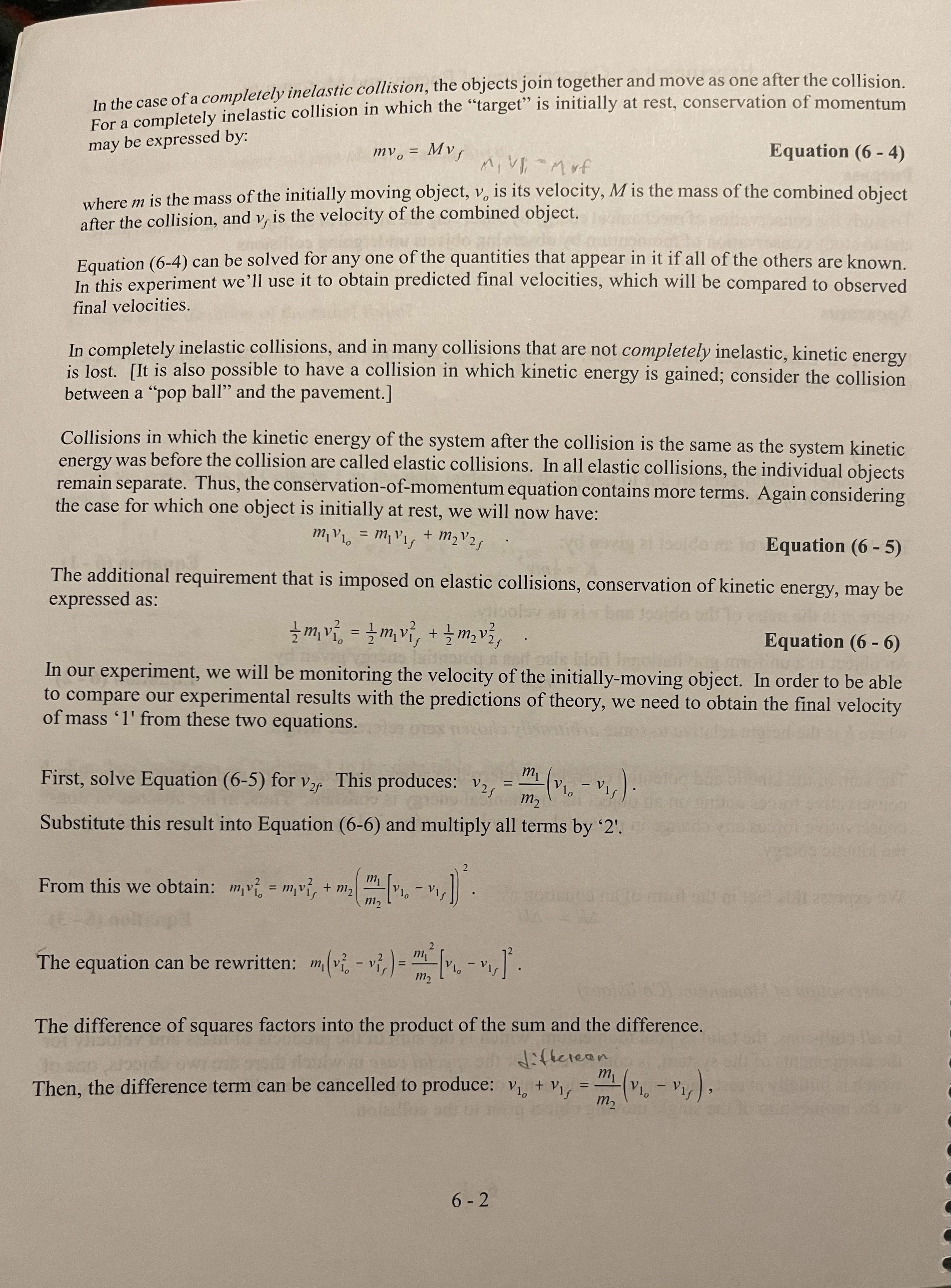
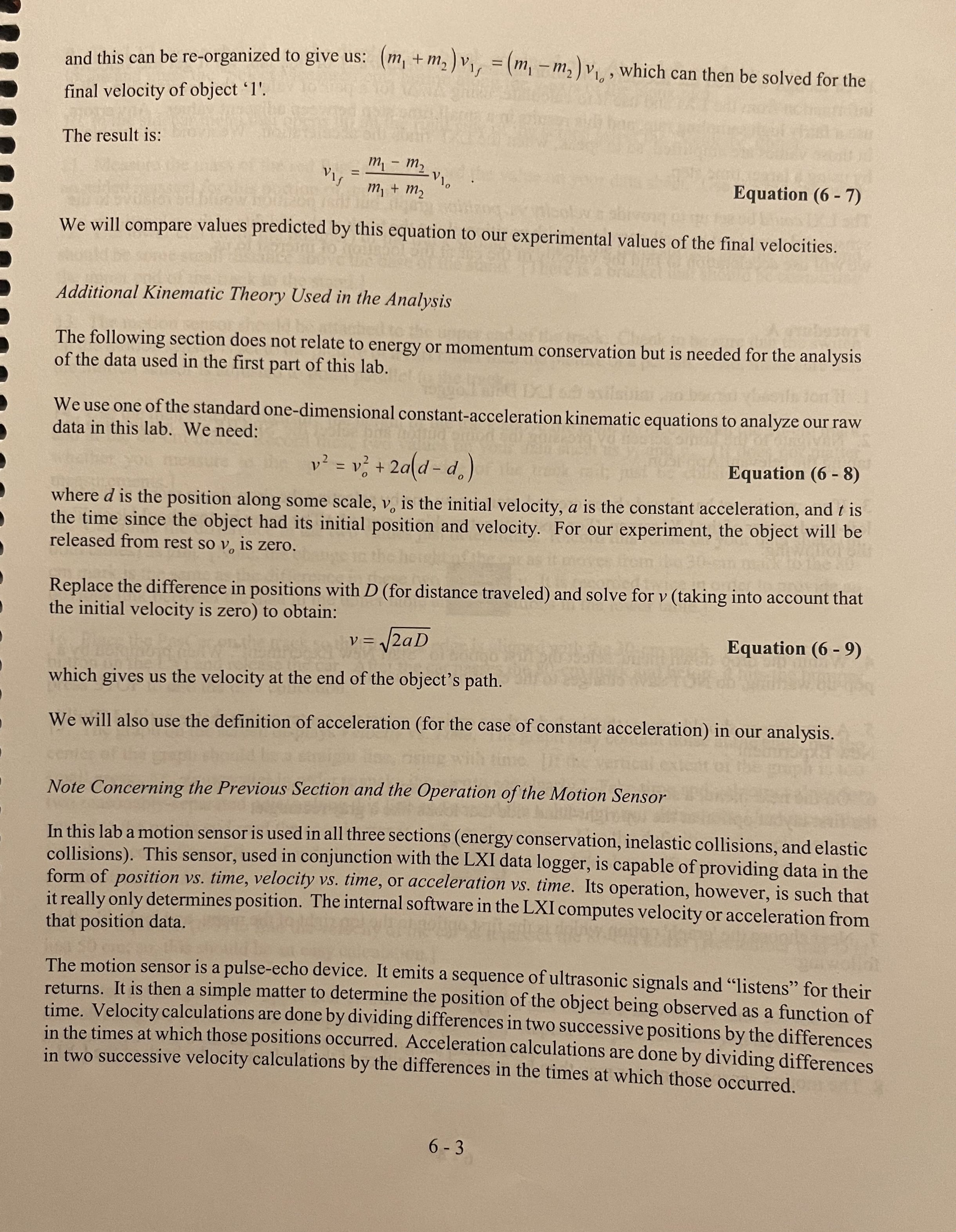
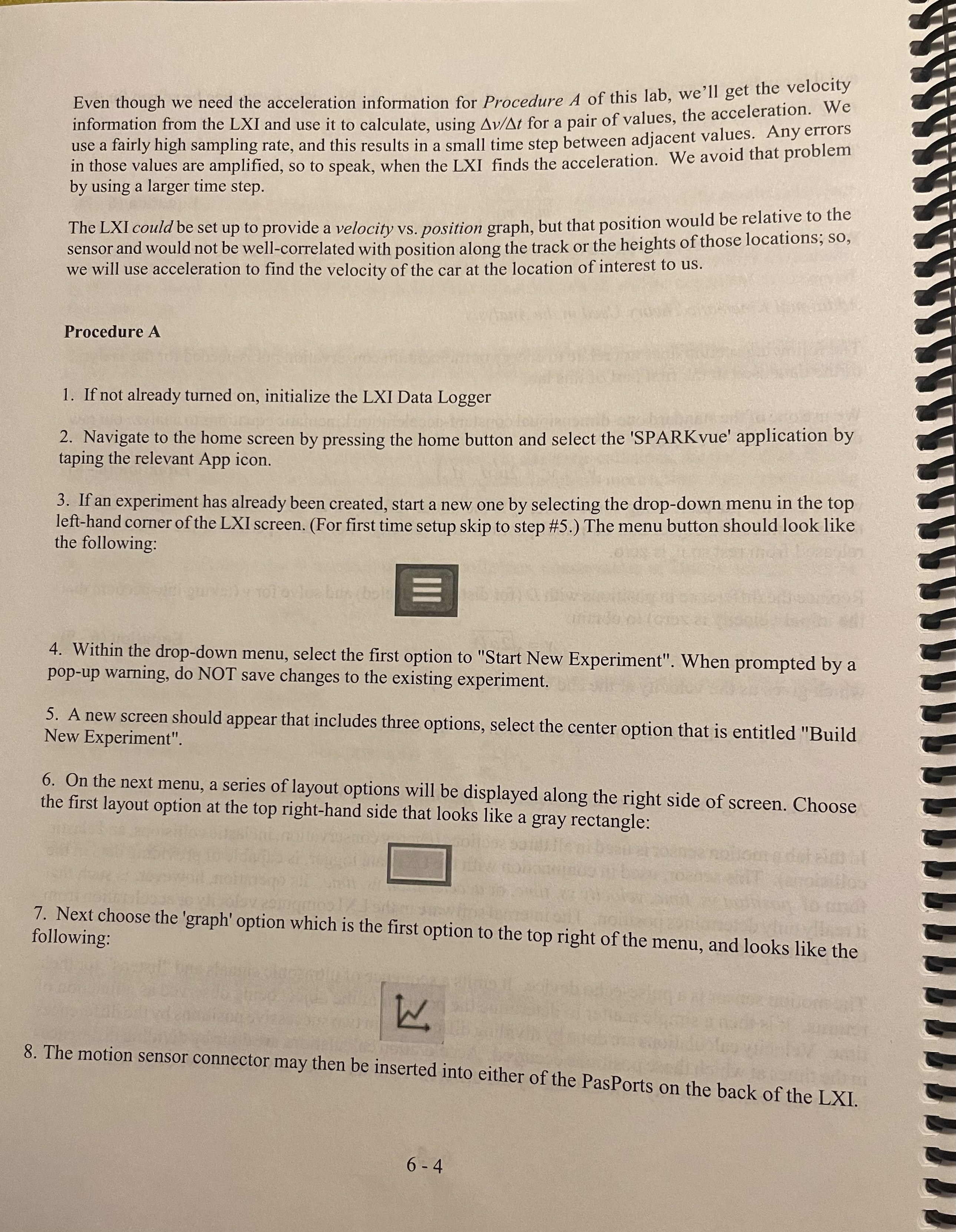
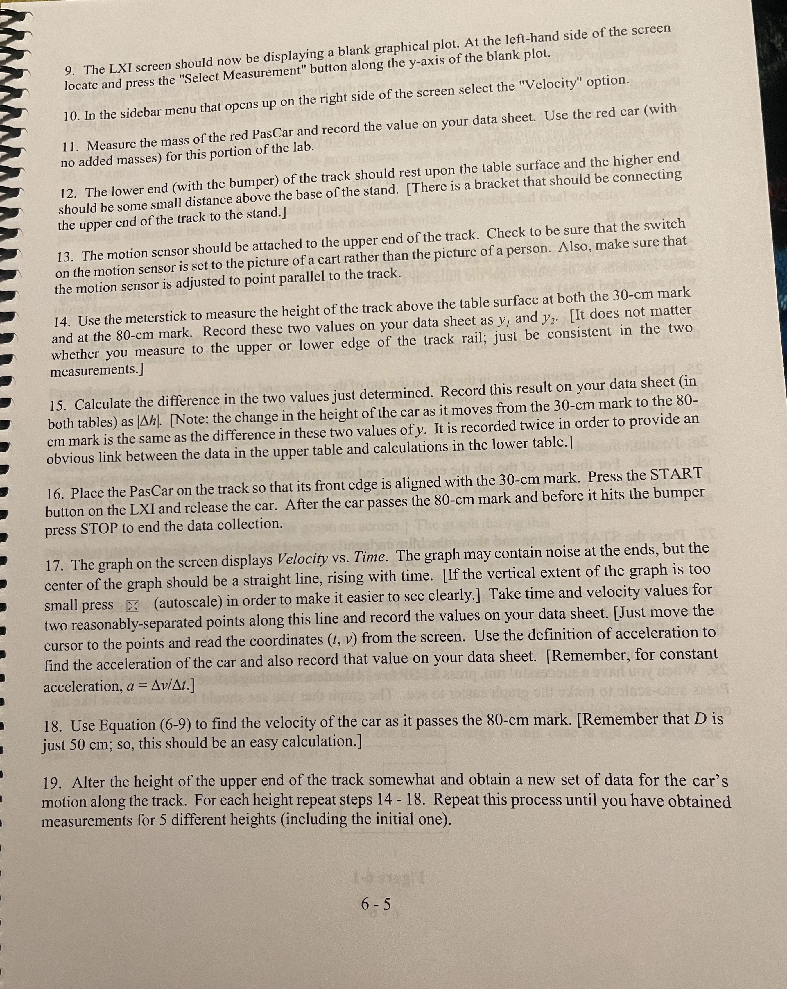
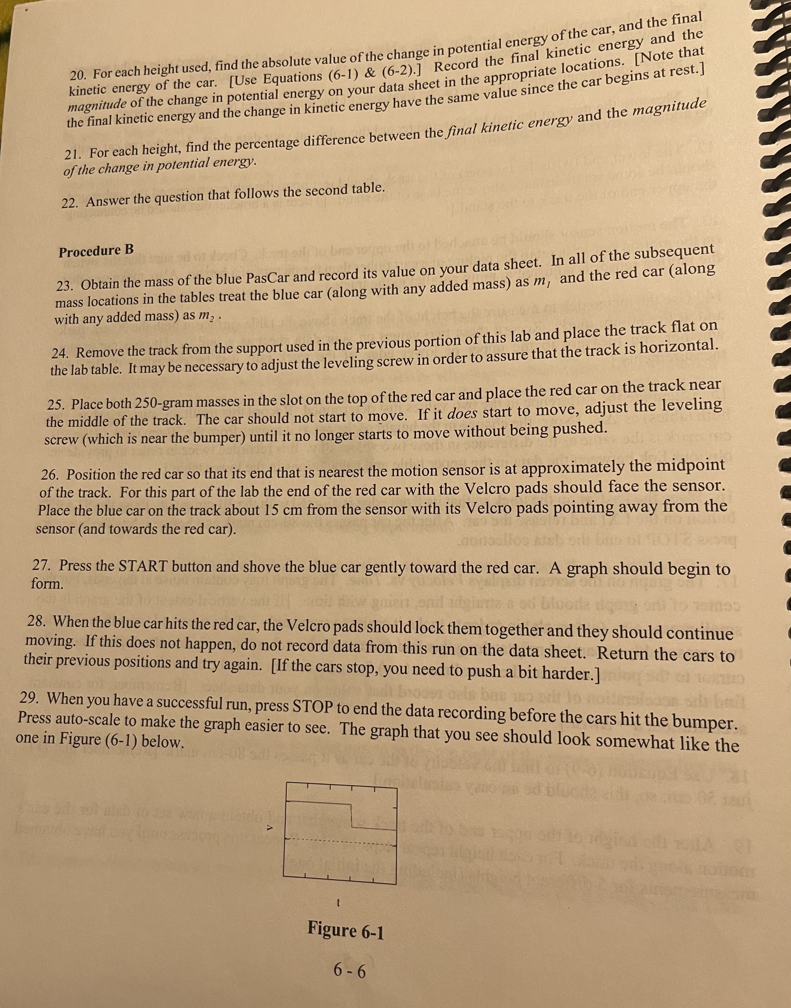
Procedure A. mass of red PasCar 254 q 1 VI V 2 (m) (m) (m) (s) (m/s) (s ) (m/s) 261 . 135 126 0 . 14 0. 65 P : 74 - 298 . 16 . 137 57 L. la 178 097 0. 45 0 .75 20 109 2 , 236 . 12 4 112 5 . 12 0. 75 0 . 65 a VS % difference (m) (m/$2 ) (m/s) (J) (J) .1126 2.4 137 J. 75 1 15 109 2 1. 77 . (12 2. 12 Ah = 41 - 72 hex = amvf V2 - V , (see related question - top of next page) a = Kf = AU VF = V2 aD 6 -9Experiment 6. Conservation of Energy and Momentum Purpose To study the conservation of mechanical energy by observing the motion of an object on an inclined plane, and to study conservation of momentum by observing objects undergoing collisions Apparatus Pasco LXI Data Logger, motion sensor, PasCars, 1.2-m dynamics track, meterstick, stand with base, electronic balance Theory Conservation of Energy The kinetic energy of an object is given by: K = Imv2 Equation (6 - 1) where m is the mass of the object and v is its velocity. An object in a uniform gravitational field also has a potential energy given by: U = mgh Equation (6 - 2) where h is the height relative to some arbitrarily chosen zero reference height. gusto .most'll essar to The sum of the kinetic and potential energies is referred to as mechanical energy and if there are no non- conservative forces acting on an object its mechanical energy is constant. Thus, in the absence of non- conservative forces any change in potential energy is accompanied by an equal and opposite change in the kinetic energy. We express this fact in the form of an equation as: AK = -AU. Equation (6 - 3) Conservation of Momentum (Collisions) In all collisions, the total system momentum, which is the sum of the products of mass and velocity for the components of the system, is conserved. For the special case in which there are two objects, one of which is initially at rest, the sum of the momenta of the two objects after the collision has the same value as the momentum of the single moving object prior to the collision. 6 - 1In the case of a completely inelastic collision, the objects join together and move as one after the collision. For a completely inelastic collision in which the "target" is initially at rest, conservation of momentum may be expressed by: my. = MVs Equation (6 - 4) where m is the mass of the initially moving object, v. is its velocity, M is the mass of the combined object after the collision, and v, is the velocity of the combined object. Equation (6-4) can be solved for any one of the quantities that appear in it if all of the others are known. In this experiment we'll use it to obtain predicted final velocities, which will be compared to observed final velocities. In completely inelastic collisions, and in many collisions that are not completely inelastic, kinetic energy is lost. [It is also possible to have a collision in which kinetic energy is gained; consider the collision between a "pop ball" and the pavement.] Collisions in which the kinetic energy of the system after the collision is the same as the system kinetic energy was before the collision are called elastic collisions. In all elastic collisions, the individual objects remain separate. Thus, the conservation-of-momentum equation contains more terms. Again considering the case for which one object is initially at rest, we will now have: wa el Boldon Equation (6 -5) The additional requirement that is imposed on elastic collisions, conservation of kinetic energy, may be expressed as: Equation (6 - 6) In our experiment, we will be monitoring the velocity of the initially-moving object. In order to be able to compare our experimental results with the predictions of theory, we need to obtain the final velocity of mass 'l' from these two equations. First, solve Equation (6-5) for vy This produces: v2, = m my ( v1 0 - VIS ) . m 2 Substitute this result into Equation (6-6) and multiply all terms by '2'. From this we obtain: mv? = mv?, + my|my [v. - vis])". The equation can be rewritten: m (vi - v],)= =[v. - vy, ]. The difference of squares factors into the product of the sum and the difference. differeen Then, the difference term can be cancelled to produce: 1 + 1 = mi (v. - Vis ) 6 -2and this can be re-organized to give us: (m, + m, ) vy, = (m, -m2 ) V1 , which can then be solved for the final velocity of object '1'. The result is: VIS mi - m2 V1. my + m2 Equation (6 - 7) We will compare values predicted by this equation to our experimental values of the final velocities. Additional Kinematic Theory Used in the Analysis The following section does not relate to energy or momentum conservation but is needed for the analysis of the data used in the first part of this lab. We use one of the standard one-dimensional constant-acceleration kinematic equations to analyze our raw data in this lab. We need: v 2 = v ?+ 2a(d-d. ) Equation (6 -8) where d is the position along some scale, v. is the initial velocity, a is the constant acceleration, and t is the time since the object had its initial position and velocity. For our experiment, the object will be released from rest so v. is zero. Replace the difference in positions with D (for distance traveled) and solve for v (taking into account that the initial velocity is zero) to obtain: v = V2aD Equation (6 - 9) which gives us the velocity at the end of the object's path. We will also use the definition of acceleration (for the case of constant acceleration) in our analysis. Note Concerning the Previous Section and the Operation of the Motion Sensor In this lab a motion sensor is used in all three sections (energy conservation, inelastic collisions, and elastic collisions). This sensor, used in conjunction with the LXI data logger, is capable of providing data in the form of position vs. time, velocity vs. time, or acceleration vs. time. Its operation, however, is such that it really only determines position. The internal software in the LXI computes velocity or acceleration from that position data. The motion sensor is a pulse-echo device. It emits a sequence of ultrasonic signals and "listens" for their returns. It is then a simple matter to determine the position of the object being observed as a function of time. Velocity calculations are done by dividing differences in two successive positions by the differences in the times at which those positions occurred. Acceleration calculations are done by dividing differences in two successive velocity calculations by the differences in the times at which those occurred. 6 - 3Even though we need the acceleration information for Procedure A of this lab, we'll get the velocity information from the LXI and use it to calculate, using Av/At for a pair of values, the acceleration. We use a fairly high sampling rate, and this results in a small time step between adjacent values. Any errors in those values are amplified, so to speak, when the LXI finds the acceleration. We avoid that problem by using a larger time step. The LXI could be set up to provide a velocity vs. position graph, but that position would be relative to the sensor and would not be well-correlated with position along the track or the heights of those locations; so, we will use acceleration to find the velocity of the car at the location of interest to us. Procedure A 1. If not already turned on, initialize the LXI Data Logger 2. Navigate to the home screen by pressing the home button and select the 'SPARK vue' application by taping the relevant App icon. 3. If an experiment has already been created, start a new one by selecting the drop-down menu in the top left-hand corner of the LXI screen. (For first time setup skip to step #5.) The menu button should look like the following: 4. Within the drop-down menu, select the first option to "Start New Experiment". When prompted by a pop-up warning, do NOT save changes to the existing experiment. 5. A new screen should appear that includes three options, select the center option that is entitled "Build New Experiment". 6. On the next menu, a series of layout options will be displayed along the right side of screen. Choose the first layout option at the top right-hand side that looks like a gray rectangle: following: 7. Next choose the 'graph' option which is the first option to the top right of the menu, and looks like the W. 8. The motion sensor connector may then be inserted into either of the PasPorts on the back of the LXI. 6 -49. The LXI screen should now be displaying a blank graphical plot. At the left-hand side of the screen locate and press the "Select Measurement" button along the y-axis of the blank plot. 10. In the sidebar menu that opens up on the right side of the screen select the "Velocity" option. 1 1. Measure the mass of the red PasCar and record the value on your data sheet. Use the red car (with no added masses) for this portion of the lab. 12. The lower end (with the bumper) of the track should rest upon the table surface and the higher end should be some small distance above the base of the stand. [There is a bracket that should be connecting the upper end of the track to the stand. ] 13. The motion sensor should be attached to the upper end of the track. Check to be sure that the switch on the motion sensor is set to the picture of a cart rather than the picture of a person. Also, make sure that the motion sensor is adjusted to point parallel to the track. 14. Use the meterstick to measure the height of the track above the table surface at both the 30-cm mark and at the 80-cm mark. Record these two values on your data sheet as y, and y2. [It does not matter whether you measure to the upper or lower edge of the track rail; just be consistent in the two measurements.] 15. Calculate the difference in the two values just determined. Record this result on your data sheet (in both tables) as |Ah). [Note: the change in the height of the car as it moves from the 30-cm mark to the 80- cm mark is the same as the difference in these two values of y. It is recorded twice in order to provide an obvious link between the data in the upper table and calculations in the lower table.] 16. Place the PasCar on the track so that its front edge is aligned with the 30-cm mark. Press the START button on the LXI and release the car. After the car passes the 80-cm mark and before it hits the bumper press STOP to end the data collection. 17. The graph on the screen displays Velocity vs. Time. The graph may contain noise at the ends, but the center of the graph should be a straight line, rising with time. [If the vertical extent of the graph is too small press (autoscale) in order to make it easier to see clearly.] Take time and velocity values for two reasonably-separated points along this line and record the values on your data sheet. [Just move the cursor to the points and read the coordinates (t, v) from the screen. Use the definition of acceleration to find the acceleration of the car and also record that value on your data sheet. [Remember, for constant acceleration, a = Av/At.] 18. Use Equation (6-9) to find the velocity of the car as it passes the 80-cm mark. [Remember that D is just 50 cm; so, this should be an easy calculation.] 19. Alter the height of the upper end of the track somewhat and obtain a new set of data for the car's motion along the track. For each height repeat steps 14 - 18. Repeat this process until you have obtained measurements for 5 different heights (including the initial one). 6- 520. For each height used, find the absolute value of the change in potential energy of the car, and the final kinetic energy of the car. [Use Equations (6-1) & (6-2).] Record the final kinetic energy and the magnitude of the change in potential energy on your data sheet in the appropriate locations. [Note that the final kinetic energy and the change in kinetic energy have the same value since the car begins at rest. ] 21. For each height, find the percentage difference between the final kinetic energy and the magnitude of the change in potential energy. 22. Answer the question that follows the second table. Procedure B 23. Obtain the mass of the blue PasCar and record its value on your data sheet. In all of the subsequent mass locations in the tables treat the blue car (along with any added mass) as m, and the red car (along with any added mass) as my . 24. Remove the track from the support used in the previous portion of this lab and place the track flat on the lab table. It may be necessary to adjust the leveling screw in order to assure that the track is horizontal. 25. Place both 250-gram masses in the slot on the top of the red car and place the red car on the track near the middle of the track. The car should not start to move. If it does start to move, adjust the leveling screw (which is near the bumper) until it no longer starts to move without being pushed. 26. Position the red car so that its end that is nearest the motion sensor is at approximately the midpoint of the track. For this part of the lab the end of the red car with the Velcro pads should face the sensor. Place the blue car on the track about 15 cm from the sensor with its Velcro pads pointing away from the sensor (and towards the red car). form. 27. Press the START button and shove the blue car gently toward the red car. A graph should begin to 28. When the blue car hits the red car, the Velcro pads should lock them together and they should continue moving. If this does not happen, do not record data from this run on the data sheet. Return the cars to their previous positions and try again. [If the cars stop, you need to push a bit harder.] 29. When you have a successful run, press STOP to end the data recording before the cars hit the bumper. Press auto-scale to make the graph easier to see. The graph that you see should look somewhat like the one in Figure (6-1) below. Figure 6-1 6 - 6