please do steps 9, 13-17 only and when finished, please post those steps only on spreadsheet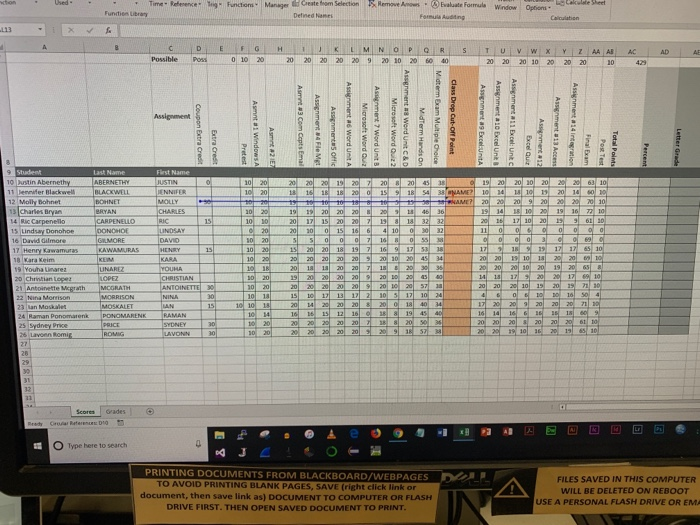

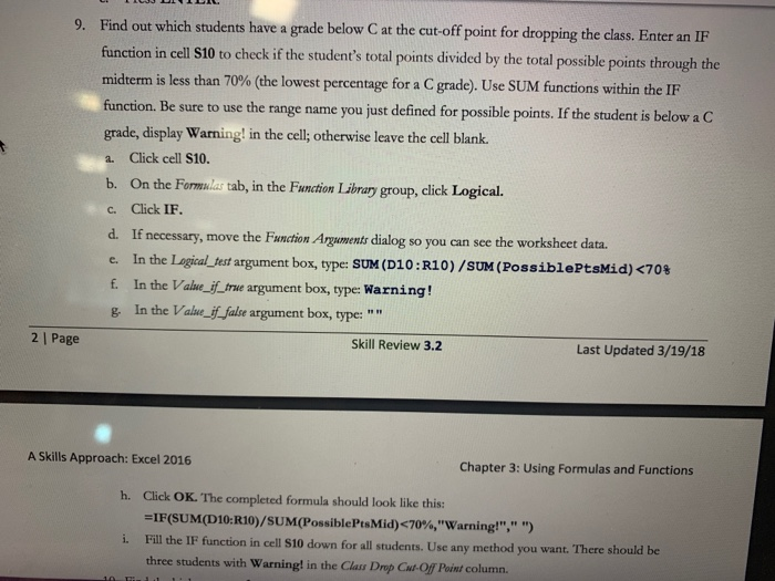
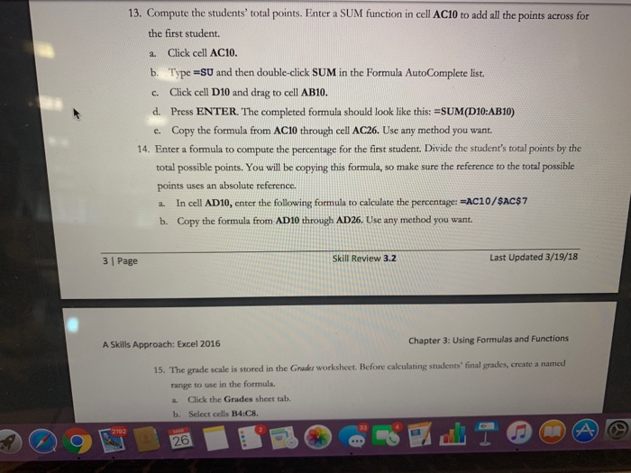
, Time-Reference* 9" Furetom. Manager tkiCreatetom Selection RemoveAnows. Evaluate Formula window Functien Libray Defined Nanmes Calculation G| H AD Possible Poss0 10 2020 20 20 20 20 9 20 0 20 60 40 20202010, 20-2020 ustin Abernethy 10 ENNIFER MOLLY NAME 16 David Gilmore 8 Kara Keim 20 Chrintian 22 Nina Morison 3 ian Moskalet eteren DO e O Type here to search PRINTING DOCUMENTS FROM BLACKBOARD/WEBPAGESP FILES SAVED IN THIS COMPUTER WILL BE DELETED ON REBOOT TO AVOID PRINTING BLANK PAGES, SAVE (right click link or document, then save link as) DOCUMENT TO COMPUTER OR FLASH DRIVE FIRST. THEN OPEN SAVED DOCUMENT TO PRINT USE A PERSONAL FLASH DRIVE OR EMA 13. Compute the students' total points. Enter a SUM function in cell AC10 to add all the points across for the first student. a. Click cell AC10. b. Type-SU and then double-click SUM in the Formula AutoComplete list. c. Click cell D10 and drag to cell AB10. d. Press ENTER. The completed formula should look like this: =SUM (D10:AB10) e. Copy the formula from AC10 through cell AC26. Use any method you want. 14. Enter a formula to compute the percentage for the first student. Divide the student's total points by the total possible points. You will be copying this formula, so make sure the reference to the total possible points uses an absolute reference. a. In cell AD10, enter the following formula to calculate the percentage: -AC10/SAC$7 b. Copy the formula from AD10 through AD26. Use any method you want. 3 | Page Skill Review 3.2 Last Updated 3/19/18 A Skills Approach: Excel 2016 Chapter 3: Using Formulas and Functions 15. The grade scale is stored in the Grakz worksheet. Before calculating students' final grades, create a named range to use in the formula. a. Click the Grades sheet tab. b. Select cells B4:C8 26 15. The grade scale is stored in the Grader worksheet. Before calculating students' final grades, create a named range to use in the formula. a. Click the Grades sheet tab. b. Select cells B4:C8. c. Type GradeScale in the Name box. d. Press ENTER. 16. Now you are ready to create a lookup formula to display each student's final letter grade. a. Return to the Scores sheet, and click cell AE10 b. On the Formulas tab, in the Funcion ibrary group, click the Lookup & Reference button, and select VLOOKUP c. Click cell AD10 to enter it in the Lookenp nalue argument box. d. Type GradeScale in the Tablk amg argument box. e. The rates are located in the second column of the lookup table. Type 2 in the Col inderc m argument box. f. In this case, you do not want to specify an exacr match, as the percentage grades do not match the grade scale percentages exactly. An approximate match will return the correct letter grade g. Click OK. The completed formula should look like this: =VLOOKUP(ADIO,GradeScale2) h. Fill down for all students. Use any method you want 17. Before closing the project, check your workbook for errors a On the Formwlar tab, in the Formala Awditing group, click the Error Checking button b. If errors are found, use the error cheeking skills learned in this chapter to find and fix the errors 18. When Excel displays a message that the error check is complete, click OK 19. Save and close the workbook Step 2 Upload & 2192 , Time-Reference* 9" Furetom. Manager tkiCreatetom Selection RemoveAnows. Evaluate Formula window Functien Libray Defined Nanmes Calculation G| H AD Possible Poss0 10 2020 20 20 20 20 9 20 0 20 60 40 20202010, 20-2020 ustin Abernethy 10 ENNIFER MOLLY NAME 16 David Gilmore 8 Kara Keim 20 Chrintian 22 Nina Morison 3 ian Moskalet eteren DO e O Type here to search PRINTING DOCUMENTS FROM BLACKBOARD/WEBPAGESP FILES SAVED IN THIS COMPUTER WILL BE DELETED ON REBOOT TO AVOID PRINTING BLANK PAGES, SAVE (right click link or document, then save link as) DOCUMENT TO COMPUTER OR FLASH DRIVE FIRST. THEN OPEN SAVED DOCUMENT TO PRINT USE A PERSONAL FLASH DRIVE OR EMA 13. Compute the students' total points. Enter a SUM function in cell AC10 to add all the points across for the first student. a. Click cell AC10. b. Type-SU and then double-click SUM in the Formula AutoComplete list. c. Click cell D10 and drag to cell AB10. d. Press ENTER. The completed formula should look like this: =SUM (D10:AB10) e. Copy the formula from AC10 through cell AC26. Use any method you want. 14. Enter a formula to compute the percentage for the first student. Divide the student's total points by the total possible points. You will be copying this formula, so make sure the reference to the total possible points uses an absolute reference. a. In cell AD10, enter the following formula to calculate the percentage: -AC10/SAC$7 b. Copy the formula from AD10 through AD26. Use any method you want. 3 | Page Skill Review 3.2 Last Updated 3/19/18 A Skills Approach: Excel 2016 Chapter 3: Using Formulas and Functions 15. The grade scale is stored in the Grakz worksheet. Before calculating students' final grades, create a named range to use in the formula. a. Click the Grades sheet tab. b. Select cells B4:C8 26 15. The grade scale is stored in the Grader worksheet. Before calculating students' final grades, create a named range to use in the formula. a. Click the Grades sheet tab. b. Select cells B4:C8. c. Type GradeScale in the Name box. d. Press ENTER. 16. Now you are ready to create a lookup formula to display each student's final letter grade. a. Return to the Scores sheet, and click cell AE10 b. On the Formulas tab, in the Funcion ibrary group, click the Lookup & Reference button, and select VLOOKUP c. Click cell AD10 to enter it in the Lookenp nalue argument box. d. Type GradeScale in the Tablk amg argument box. e. The rates are located in the second column of the lookup table. Type 2 in the Col inderc m argument box. f. In this case, you do not want to specify an exacr match, as the percentage grades do not match the grade scale percentages exactly. An approximate match will return the correct letter grade g. Click OK. The completed formula should look like this: =VLOOKUP(ADIO,GradeScale2) h. Fill down for all students. Use any method you want 17. Before closing the project, check your workbook for errors a On the Formwlar tab, in the Formala Awditing group, click the Error Checking button b. If errors are found, use the error cheeking skills learned in this chapter to find and fix the errors 18. When Excel displays a message that the error check is complete, click OK 19. Save and close the workbook Step 2 Upload & 2192