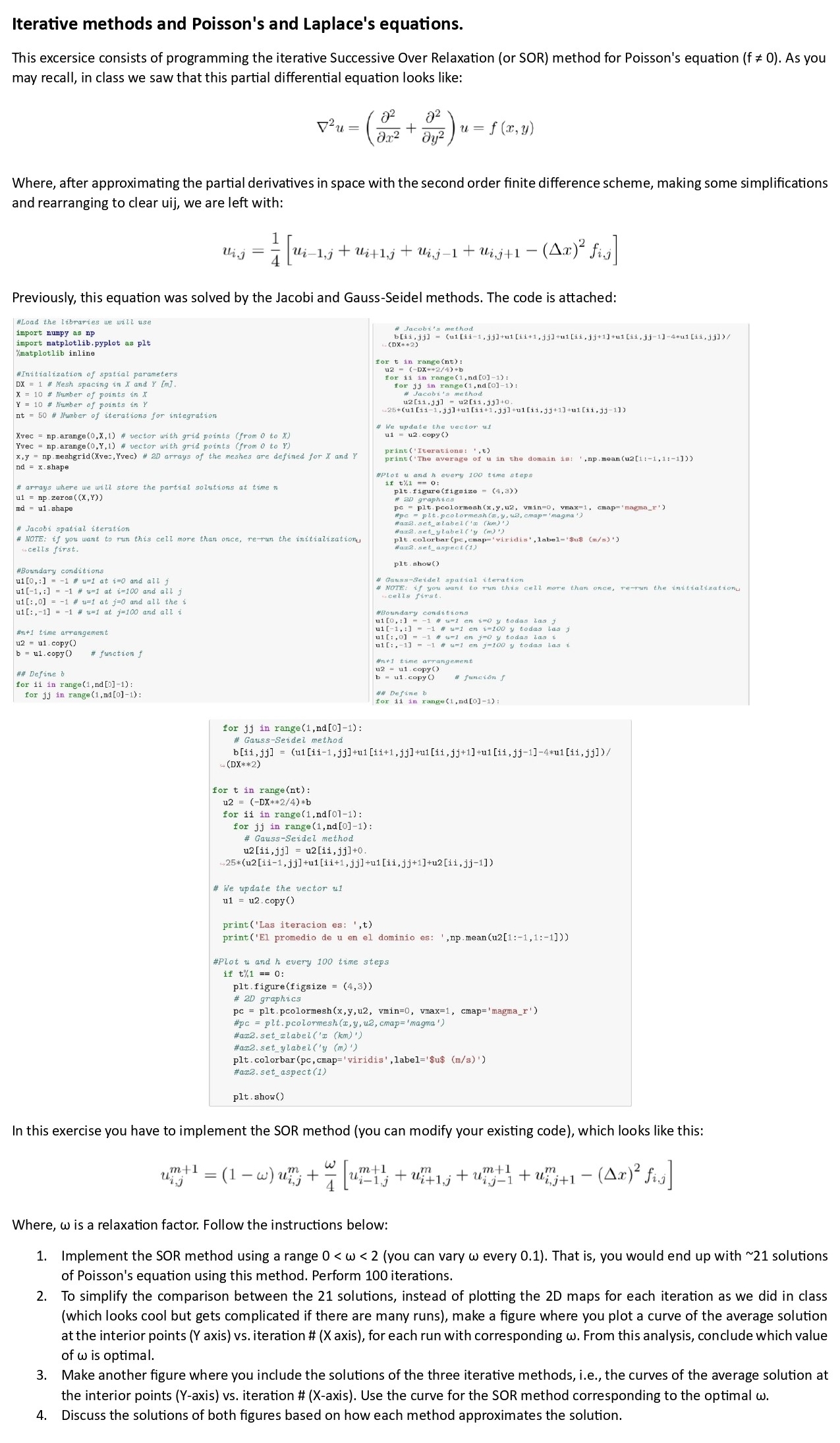
Please do this excersise in Python

Iterative methods and Poisson's and Laplace's equations. This excersice consists of programming the iterative Successive Over Relaxation (or SOR) method for Poisson's equation (f O). As you may recall, in class we saw that this partial differential equation looks like: 02 v2u= Dx2 02 D!J2 Where, after approximating the partial derivatives in space with the second order finite difference scheme, making some simplifications and rearranging to clear uij, we are left with: 1 + Ui+l,j -+- 4- (Ax) 2 4 Previously, this equation was solved by the Jacobi and Gauss-Seidel methods. The code is attached: *Load the use import numpy as np import matplotlib.pypLot as pit Vanatplotlib inline spatial parameters X I # Mesh X and Y X 10 # "umber of points X Y 10 * Of Y Xvec = # vector points (from O to X) Yvec 4 oector with grid points (from O to Y) x, y = arrays of the meshes defined for X and nd x. shape # we store the solutions at tine n ul md = ul ehape Jacobi spat i a I NOTE: if you to run this cell than once, the ulto,: ul[-l,;] ult:, -I at and at L j 1 the i -1 at and u2 ul . copy() b ul.copy() # function f Define b for Ii in for jj in range(l bi's . eopy( ) print The u and h 100 time seeps pit . an graphic: MOTE; y todas 2 - copyo for .ndtoj-l) : for jj in # GaussSeidel method (ul [ii- 1, jj]+ul Cii+l , jj]+ul [ii,jj+l] [ii,jj- for t in range(nt): u2 = for ii in for jj in # GaussSeidel method 25* (u2 [iil , jj] +uI Cii+l , jj] +ul [ii , j j +1]+u2 Cii , jjI] ) # We update the oector ul ul = u2.copy() print('Las iteracion es: print('E1 promedio de u en u and every 100 time if t'/.l O p1t . figure (figsize = # 21) graphics eI dominio es: s t eps , np. mean (u2 C pc = p1t.pc010rmesh(x,y,u2, vmin=O, vmax=l, ) = cmap='magma ' ) #a2. set _ ylabel('y (n) ' ) plt . colorbar viridis' , label='$u$ (m/s) ) #ac2. set_aspect(l) pit . show() In this exercise you have to implement the SOR method (you can modify your existing code), which looks like this: In-Fl Where, w is a relaxation factor. Follow the instructions below: 1. 2. 3. 4. Implement the SOR method using a range O < w < 2 (you can vary w every 0.1). That is, you would end up with N 21 solutions of Poisson's equation using this method. Perform 100 iterations. To simplify the comparison between the 21 solutions, instead of plotting the 2D maps for each iteration as we did in class (which looks cool but gets complicated if there are many runs), make a figure where you plot a curve of the average solution at the interior points (Y axis) vs. iteration # (X axis), for each run with corresponding w. From this analysis, conclude which value of w is optimal. Make another figure where you include the solutions of the three iterative methods, i.e., the curves of the average solution at the interior points (Y-axis) vs. iteration # (X-axis). Use the curve for the SOR method corresponding to the optimal w. Discuss the solutions of both figures based on how each method approximates the solution.