Question: please explain in details:- Criminologists have long debated whether there is a relationship between weather conditions and the incidence of violent crime. The author of
please explain in details:-


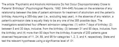
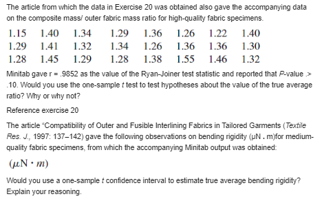
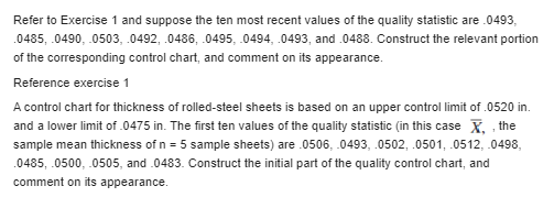
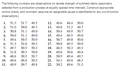
Criminologists have long debated whether there is a relationship between weather conditions and the incidence of violent crime. The author of the article "Is There a Season for Homicide?" (Criminology, 1988: 287-296) classified 1361 homicides according to season, resulting in the accompanying data. Test the null hypothesis of equal proportions using a = .01 by using the chi-squared table to say as much as possible about the P-value. 0 = .01The article "Psychiatric and Alcoholic Admissions Do Not Occur Disproportionately Close to Patients' Birthdays" (Psychological Reports. 1092: 944-946) focuses on the existence of any relationship between the date of patient admission for treatment of alcoholism and the patient's birthday. Assuming a 365-day year (i.e., excluding leap year), in the absence of any relation, a patient's admission date is equally likely to be any one of the 365 possible days. The investigators established four different admission categories: (1) within 7 days of birthday: (2) between 8 and 30 days, inclusive, from the birthday: (3) between 31 and 90 days, inclusive, from the birthday; and (4) more than 90 days from the birthday. A sample of 200 patients gave observed frequencies of 11, 24, 60. and 06 for categories 1, 2. 3, and 4, respectively. State and test the relevant hypotheses using a significance level of .01.The article from which the data in Exercise 20 was obtained also gave the accompanying data on the composite mass/ outer fabric mass ratio for high-quality fabric specimens. 1.15 1.40 1.34 1.29 1.36 1.26 1.22 1.40 1.29 1.41 1.32 1.34 1.26 1 1.36 1.36 1.30 1.28 1.45 1.29 1.28 1.38 1.55 1.46 1.32 Minitab gave r = .9852 as the value of the Ryan-Joiner test statistic and reported that P-value .> .10. Would you use the one-sample t test to test hypotheses about the value of the true average ratio? Why or why not? Reference exercise 20 The article "Compatibility of Outer and Fusible Interlining Fabrics in Tailored Garments (Textile Res. J., 1997: 137-142) gave the following observations on bending rigidity (UN . m)for medium- quality fabric specimens, from which the accompanying Minitab output was obtained: (UN . m) Would you use a one-sample t confidence interval to estimate true average bending rigidity? Explain your reasoning.A control chart for thickness of rolled-steel sheets is based on an upper control limit of .0520 in. and a lower limit of .0475 in. The first ten values of the quality statistic (in this case X. , the sample mean thickness of n = 5 sample sheets) are .0506, _0493, .0502, .0501, .0512, .0498, 0485, .0500, _0505, and .0483. Construct the initial part of the quality control chart, and comment on its appearance.Refer to Exercise 1 and suppose the ten most recent values of the quality statistic are .0493, 0485, .0490, 0503, .0492, .0486, .0495, 0494, .0493, and .0488. Construct the relevant portion of the corresponding control chart, and comment on its appearance. Reference exercise 1 A control chart for thickness of rolled-steel sheets is based on an upper control limit of . 0520 in. and a lower limit of .0475 in. The first ten values of the quality statistic (in this case X. , the sample mean thickness of n = 5 sample sheets) are .0506, _0493, .0502, . 0501, .0512, .0498, 0485, .0500, 0505, and .0483. Construct the initial part of the quality control chart, and comment on its appearance.Calculate control limits for the data of Exercise 8 using the robust procedure presented in this section. Reference exercise 8 The table below gives data on moisture content for specimens of a certain type of fabric. Determine control limits for a chart with center line at height 13.00 based on o = .600, construct the control chart, and comment on its appearance. D = .600.A manufacturer of dustless chalk instituted a quality control program to monitor chalk density. The sample standard deviations of densities for 24 different subgroups, each consisting n = 8 of chalk specimens, were as follows: 204 .315 .096 .184 230 .212 .322 .287 145 .211 .053 .145 .272 .351 .159 .214 .388 .187 .150 .229 .276 .118 .091 -056 Calculate limits for an S chart, construct the chart, and check for out-of-control points. If there is an out-of-control point, delete it and repeat the processContainers of a certain treatment for septic tanks are supposed to contain 16 oz of liquid. A sample of five containers is selected from the production line once each hour, and the sample average content is determined. Consider the following results: 15.992, 16.051, 16.065, 15.912, 18.030, 18.080, 15.982. 15.890, 18.038, 16.074, 16.029. 15.935, 18.032, 15.960, 16.055. Using A and h = .20, employ the computational form of the CUSUM procedure to investigate the behavior of this process.The target value for the diameter of a certain type of driveshaft is .75 in. The size of the shift in the average diameter considered important to detect is .002 in. Sample average diameters for successive groups of n = 4 shafts are as follows: .7507, .7504. .7492. .7501. .7503, .7510. .7490. 7497. . 7488. .7504. .7516. 7472. .7489. .7483, .7471. .7498. .7460, .7482, 7470. . 7493. .7482. 7481. Use the computational form of the CUSUM procedure with h = .003 to see whether the process mean remained on target throughout the time of observation.The following numbers are observations on tensile strength of synthetic fabric specimens selected from a production process at equally spaced time intervals. Construct appropriate control charts, and comment (assume an assignable cause is identifiable for any out-of-control observations). 1. 51.3 51.7 49.5 12. 496 48.4 50.0 2. 51.0 50.0 49.3 13. 49.8 51.2 49.7 3. 50.8 51.1 4910 14. 50.4 49.9 50.7 4. 50.6 51.1 15. 49.4 49.5 49.0 5. 49.6 50.5 50.9 16. 50.7 49.0 50.0 51.3 52.0 50.3 17. 50.8 49.5 50.9 7. 49.7 50.5 50.3 18. 48.5 50.3 49.3 8. 51.8 50.3 50.0 19. 49.6 50.6 49.4 48.6 50.5 50.7 20. 50.9 49.4 49.7 10. 49.6 49.8 50.5 21. 54.1 49.8 48.5 11. 49.9 50.7 49.8 22. 50.2 49.6 51.5An alternative to the p chart for the fraction defective is the no chart for number defective This chart has UCL = UCL = ap + 3Vap(1 - p). LCL = ap - 3Vap(1 - p) + 3V mp(1 - p). LCL = mp - 3 V mp(1 - p), and the number of defectives from each sample is plotted on the chart. Construct such a chart for the data of Example 18.8. Will the use of an no chart always give the same message as the use of a p chart (Le., are the two charts equivalent)
Step by Step Solution
There are 3 Steps involved in it

Get step-by-step solutions from verified subject matter experts


