

Please explain this section step by step, I am unclear in all these graphs and what is it trying to say, any try thanks !
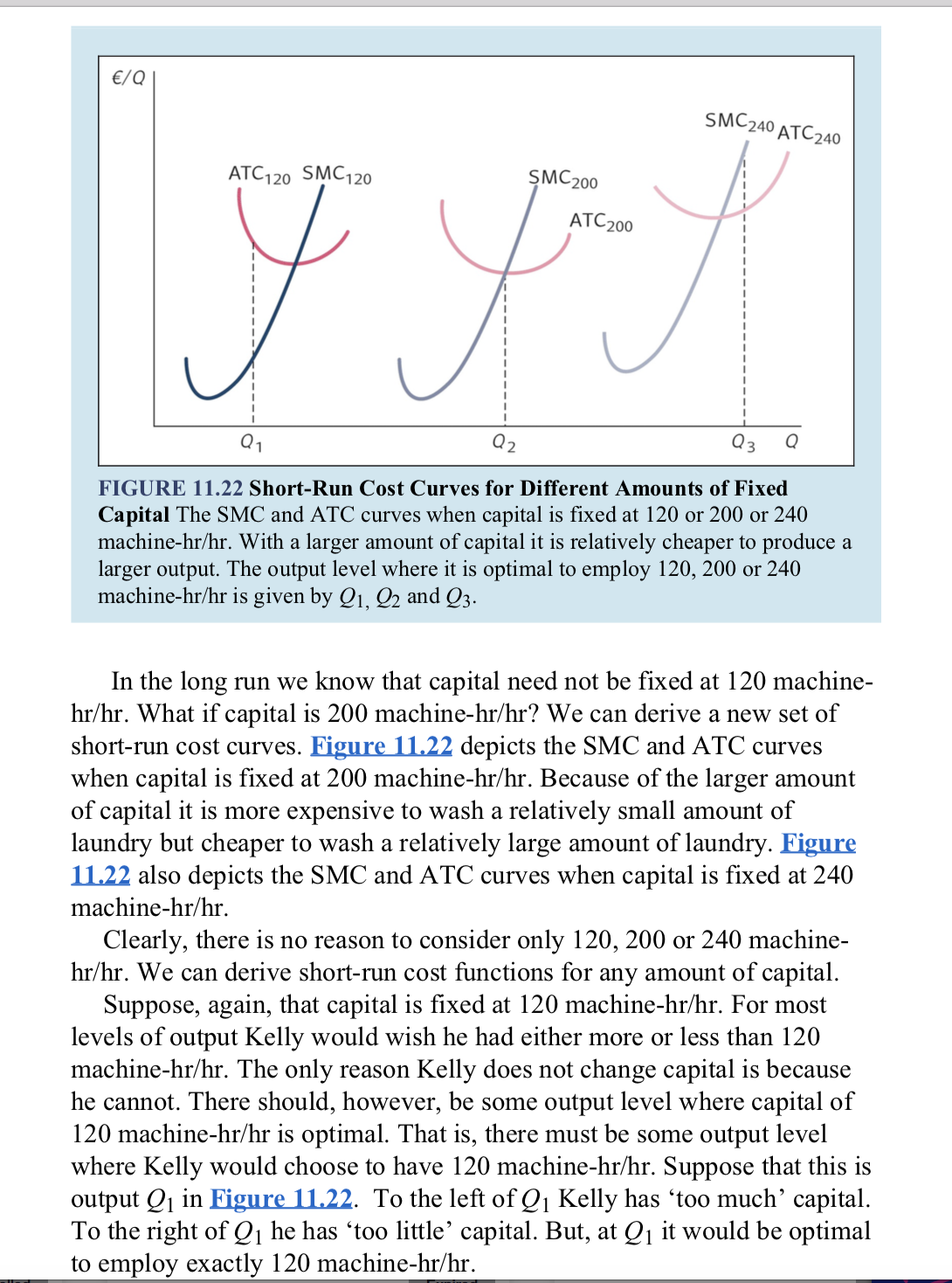
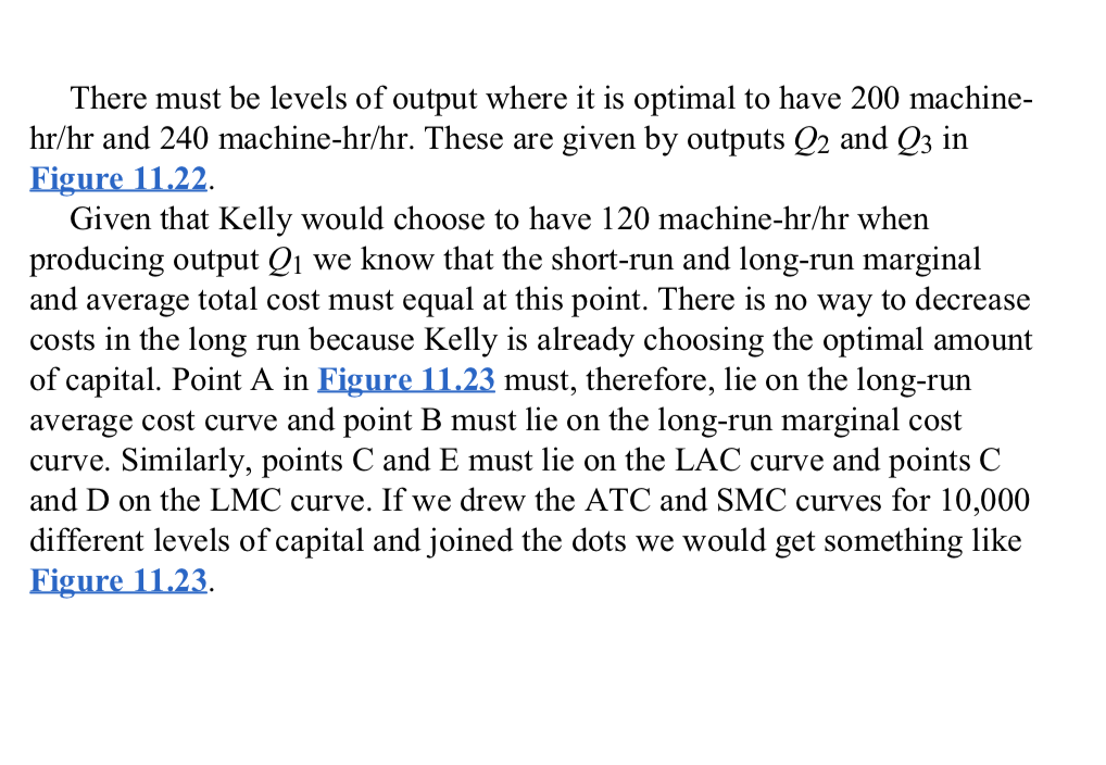
ATC120 S\"\"3120 FIGURE 11.22 Short-Run Cost Curves for Different Amounts of Fixed Capital The SMC and ATC curves when capital is xed at 120 or 200 or 240 machine-hr/hr. With a larger amount of capital it is relatively cheaper to produce a larger output. The output level where it is optimal to employ 120, 200 or 240 machine-hr/hr is given by Q1, Q2 and Q3. In the long run we know that capital need not be fixed at 120 machine hr/hr. What if capital is 200 machinehr/hr? We can derive a new set of shortrun cost curves. EignnLILZZ depicts the SMC and ATC curves when capital is fixed at 200 machinehr/hr. Because of the larger amount of capital it is more expensive to wash a relatively small amount of laundry but cheaper to wash a relatively large amount of laundry. Eigune 1122 also depicts the SMC and ATC curves when capital is fixed at 240 machine-hr/hr. Clearly, there is no reason to consider only 120, 200 or 240 machine- hr/hr. We can derive short-run cost functions for any amount of capital. Suppose, again, that capital is fixed at 120 machinehr/hr. For most levels of output Kelly would wish he had either more or less than 120 machine-hr/hr. The only reason Kelly does not change capital is because he cannot. There should, however, be some output level where capital of 120 machinehr/hr is optimal. That is, there must be some output level where Kelly would choose to have 120 machinehr/hr. Suppose that this is output Q1 in W. To the left of Q1 Kelly has 'too much' capital. To the right of Q1 he has 'too little' capital. But, at Q] it would be optimal to employ exactly 120 machine-hr/hr. There must be levels of output where it is optimal to have 200 machine hr/hr and 240 machinehr/hr. These are given by outputs Q2 and Q3 in EignmlLZZ. Given that Kelly would choose to have 120 machinehr/hr when producing output Q1 we know that the shortrun and longrun marginal and average total cost must equal at this point. There is no way to decrease costs in the long run because Kelly is already choosing the optimal amount of capital. Point A in EignmlLZl must, therefore, lie on the longrun average cost curve and point B must lie on the long-run marginal cost curve. Similarly, points C and E must lie on the LAC curve and points C and D on the LMC curve. If we drew the ATC and SMC curves for 10,000 different levels of capital and joined the dots we would get something like EIgnLLILZIi. E/Q SMC240 ATC120 SMC120 SMC 200 ATC 240 ATC 200 IE C LAC B LMC Q1 Q2 Q3 Q FIGURE 11.23 The Family of Cost Curves Associated with a U-Shaped LAC The LAC curve is the 'outer envelope' of the ATC curves. LMC = SMC at the Q value for which the ATC is tangent to the LAC. At the minimum point on the LAC, LMC = SMC = ATC = LAC. This allows us to relate short-run and long-run cost curves. There is just one more thing to mention. If Kelly is employing 120 machine-hr/hr and not producing output Q1 then his costs must be higher than they could be in the long run, because he is employing either too much or too little capital. The ATC 120 curve must, therefore, lie above the LAC curve everywhere except at 91. Similarly the ATC200 curve must lie above the LAC curve everywhere except at 92. One way of thinking of the LAC curve is thus as an 'envelope' of all the short-run average total cost curves. Note that at the minimum point on the LAC curve in Figure 11.23 (Q = Q2), the long-run and short-run marginal and average costs all take exactly the same value. The Appendix to this chapter considers the relationship between long- run and short-run costs in greater detail. It also develops the calculus approach to cost minimization


