please help
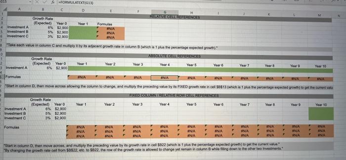
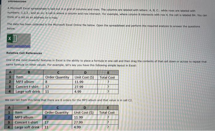
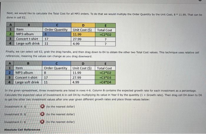
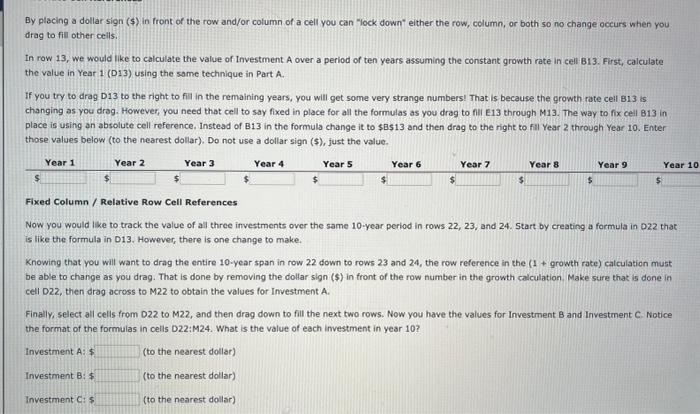
A Microsoft Excel spreadsheet is laid out in a grid of columns and rows. The columns are labeled with letters: A, B, C. while rows are labeled with numbers: 1,2,3.. and so on. A cell is where a column and row intersect. For example, where column B intersects with row 4 , the cell is labeled B4. You can think of a cell as an address on a map. The data has been collected in the Microsoft Excel Online flle below, Open the spreadsheet and perform the required analysis to answer the questions below. Relative Cell References One of the most powerful features in Excel is the ability to place a formula in one celi and then drag the contents of that cell down or across to repeat that same formula on other values. For example, let's say you have this following simple layout in Excel: We can tell from this table that there are 8 orders for the MP3 album and that value is in cell C2. Next, we would like to calculate the Total Cost for all MP3 orders. To do that we would multiply the Order Quantity by the Unit Cost; 8 * 11.99. That can bo done in cell E2. Finally, we can select cell E2, grab the drag handle, and then drag down to E4 to obtain the other two Total Cost values. This technique uses refative cell references, meaning the values can change as you drag downward. In the given spreadsheet, three investments are listed in rows 4-6. Column B contains the expected growth rate for each investment as a percentage. Calculate the expected value of Investment A in cell D4 by multiplying its value in Year 0 by the quantity (1+ Growth rate). Then drag cell D4 down to D6 to get the other two investment values after one year given different growth rates and place those values below: Investment A:1 (to the nearest dollar) Investment B: 1 Q3) (to the nearest dollar) Inventment C: (6) (to the nearest dollar) Absolute Cell References By placing a dollar sign (\$) in front of the row and/or column of a cell you can "lock down" either the row, column, or both so no change occurs when you drag to fill other ceils. In row 13, we would like to calculate the value of Investment A over a period of ten years assuming the constant growth rate in cell-B13. First, calculate the value in Year 1 (D13) using the same technique in Part A. If you try to drag D13 to the right to fill in the remaining years, you will get some very strange numbers! That is because the growth rate cell B13 is changing as you drag. However, you need that cell to say fixed in place for all the formulas as you drag to fil E13 through M13. The way to fix cell B13 in place is using an absolute cell reference. Instead of B13 in the formula change it to $8s13 and then drag to the right to fill Year 2 through Year 10 . Enter those values below (to the nearest dollar). Do not use a dollar sign (\$), just the value. Fixed Column / Relative Row Cell References Now you would ike to track the value of all three investments over the same 10 -year period in rows 22, 23, and 24. Start by creating a formula in D22 that: is like the formula in D13. However, there is one change to make. Knowing that you will want to drag the entire 10-year span in row 22 down to rows 23 and 24 , the row reference in the ( 1+ growth rate) calculation must be able to change as you drag. That is done by removing the dollar sign (\$) in front of the row number in the growth calculation, Make sure that is done in cell D22, then drag across to M22 to obtain the values for Investment A. Finaly, select all cells from D22 to M22, and then drag down to fill the next two rows. Now you have the values for Investment B and Investment C. Notice the format of the formulas in celis D22:M24. What is the value of each investment in year 10 ? investment A:{ (to the nearest dollar) Investment B:9 (to the nearest dollar) Investment C:9 (to the nearest dollar)