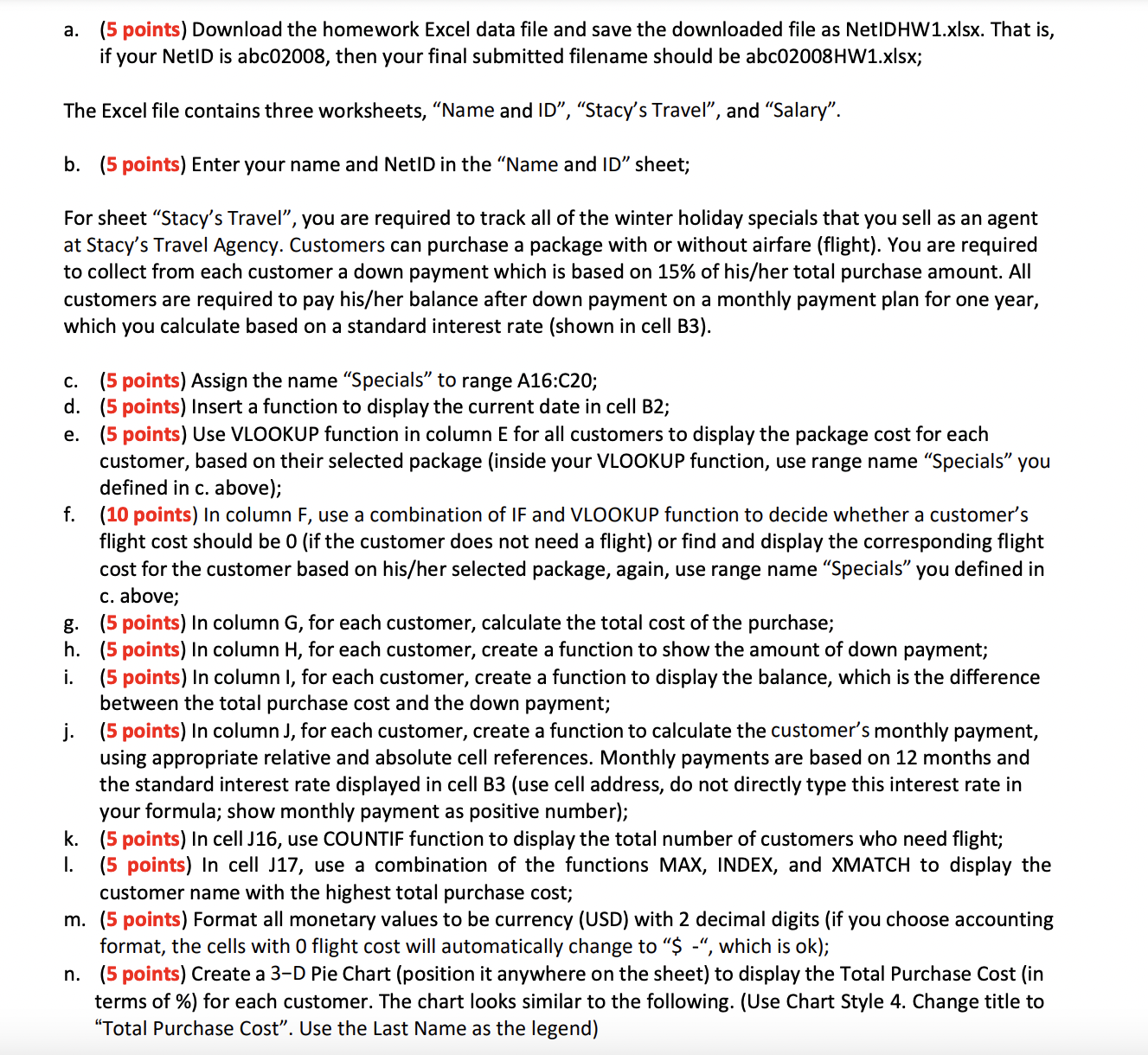
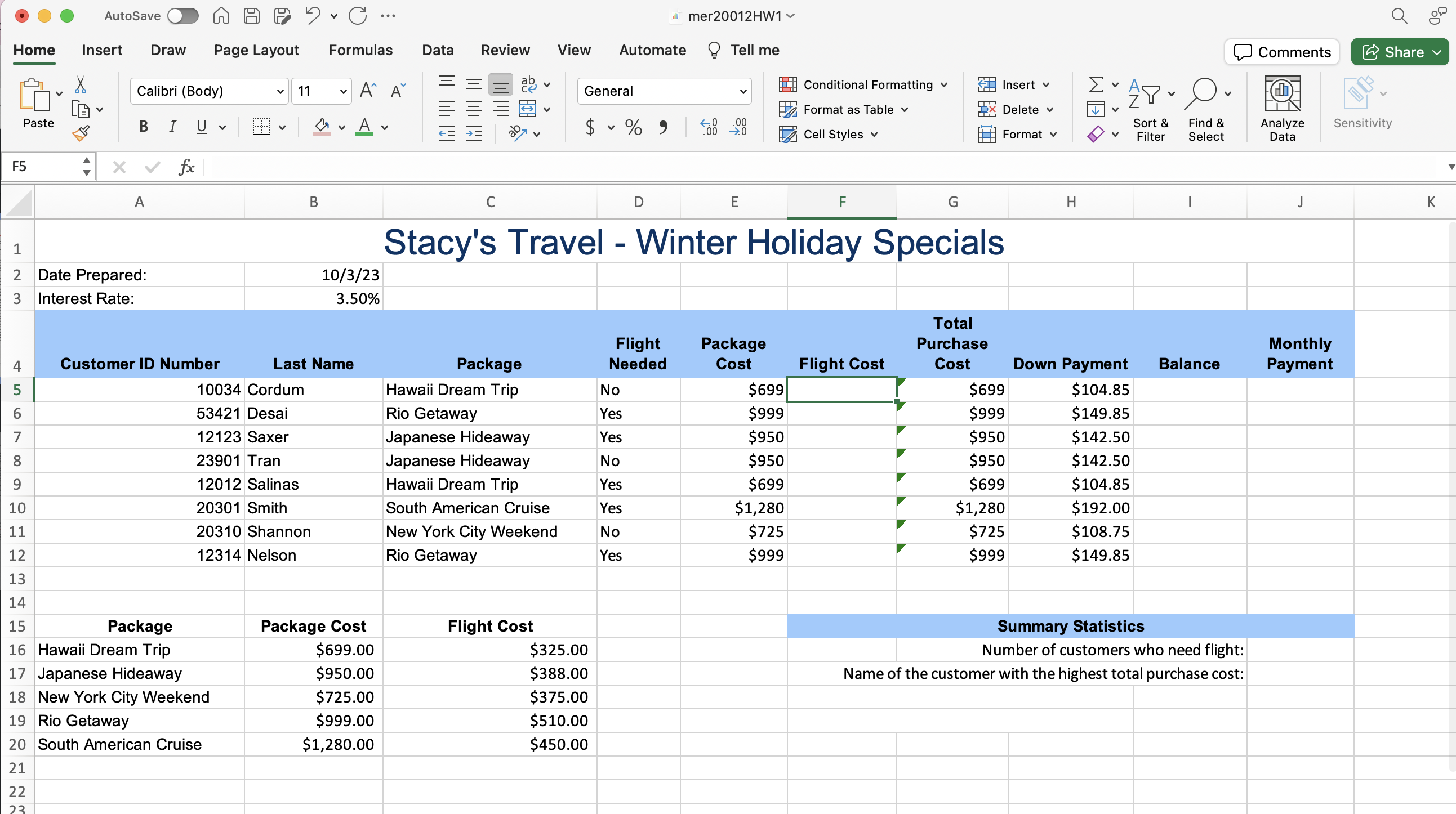
Please help me find the formula for question f!! :)

Disregard the columns for total purchase down and down payment

a. (5 points) Download the homework Excel data file and save the downloaded file as NetIDHW1.xlsx. That is, if your NetID is abc02008, then your final submitted filename should be abc02008HW1.xIsx; The Excel file contains three worksheets, "Name and ID", "Stacy's Travel", and "Salary". b. (5 points) Enter your name and NetID in the "Name and ID" sheet; For sheet "Stacy's Travel", you are required to track all of the winter holiday specials that you sell as an agent at Stacy's Travel Agency. Customers can purchase a package with or without airfare (flight). You are required to collect from each customer a down payment which is based on 15% of his/her total purchase amount. All customers are required to pay his/her balance after down payment on a monthly payment plan for one year, which you calculate based on a standard interest rate (shown in cell B3). c. (5 points) Assign the name "Specials" to range A16:C20; d. (5 points) Insert a function to display the current date in cell B2; e. (5 points) Use VLOOKUP function in column E for all customers to display the package cost for each customer, based on their selected package (inside your VLOOKUP function, use range name "Specials" you defined in c. above); f. (10 points) In column F, use a combination of IF and VLOOKUP function to decide whether a customer's flight cost should be 0 (if the customer does not need a flight) or find and display the corresponding flight cost for the customer based on his/her selected package, again, use range name "Specials" you defined in c. above; g. (5 points) In column G, for each customer, calculate the total cost of the purchase; h. (5 points) In column H, for each customer, create a function to show the amount of down payment; i. (5 points) In column I, for each customer, create a function to display the balance, which is the difference between the total purchase cost and the down payment; j. (5 points) In column J, for each customer, create a function to calculate the customer's monthly payment, using appropriate relative and absolute cell references. Monthly payments are based on 12 months and the standard interest rate displayed in cell B3 (use cell address, do not directly type this interest rate in your formula; show monthly payment as positive number); k. (5 points) In cell J16, use COUNTIF function to display the total number of customers who need flight; I. (5 points) In cell J17, use a combination of the functions MAX, INDEX, and XMATCH to display the customer name with the highest total purchase cost; m. (5 points) Format all monetary values to be currency (USD) with 2 decimal digits (if you choose accounting format, the cells with 0 flight cost will automatically change to "\$ -", which is ok); n. (5 points) Create a 3-D Pie Chart (position it anywhere on the sheet) to display the Total Purchase Cost (in terms of \%) for each customer. The chart looks similar to the following. (Use Chart Style 4. Change title to "Total Purchase Cost". Use the Last Name as the legend) a. (5 points) Download the homework Excel data file and save the downloaded file as NetIDHW1.xlsx. That is, if your NetID is abc02008, then your final submitted filename should be abc02008HW1.xIsx; The Excel file contains three worksheets, "Name and ID", "Stacy's Travel", and "Salary". b. (5 points) Enter your name and NetID in the "Name and ID" sheet; For sheet "Stacy's Travel", you are required to track all of the winter holiday specials that you sell as an agent at Stacy's Travel Agency. Customers can purchase a package with or without airfare (flight). You are required to collect from each customer a down payment which is based on 15% of his/her total purchase amount. All customers are required to pay his/her balance after down payment on a monthly payment plan for one year, which you calculate based on a standard interest rate (shown in cell B3). c. (5 points) Assign the name "Specials" to range A16:C20; d. (5 points) Insert a function to display the current date in cell B2; e. (5 points) Use VLOOKUP function in column E for all customers to display the package cost for each customer, based on their selected package (inside your VLOOKUP function, use range name "Specials" you defined in c. above); f. (10 points) In column F, use a combination of IF and VLOOKUP function to decide whether a customer's flight cost should be 0 (if the customer does not need a flight) or find and display the corresponding flight cost for the customer based on his/her selected package, again, use range name "Specials" you defined in c. above; g. (5 points) In column G, for each customer, calculate the total cost of the purchase; h. (5 points) In column H, for each customer, create a function to show the amount of down payment; i. (5 points) In column I, for each customer, create a function to display the balance, which is the difference between the total purchase cost and the down payment; j. (5 points) In column J, for each customer, create a function to calculate the customer's monthly payment, using appropriate relative and absolute cell references. Monthly payments are based on 12 months and the standard interest rate displayed in cell B3 (use cell address, do not directly type this interest rate in your formula; show monthly payment as positive number); k. (5 points) In cell J16, use COUNTIF function to display the total number of customers who need flight; I. (5 points) In cell J17, use a combination of the functions MAX, INDEX, and XMATCH to display the customer name with the highest total purchase cost; m. (5 points) Format all monetary values to be currency (USD) with 2 decimal digits (if you choose accounting format, the cells with 0 flight cost will automatically change to "\$ -", which is ok); n. (5 points) Create a 3-D Pie Chart (position it anywhere on the sheet) to display the Total Purchase Cost (in terms of \%) for each customer. The chart looks similar to the following. (Use Chart Style 4. Change title to "Total Purchase Cost". Use the Last Name as the legend)